Part 1 - Convolutional Neural Networks (CNNs)
1.1 Motivation - Why Not a Standard MLP?
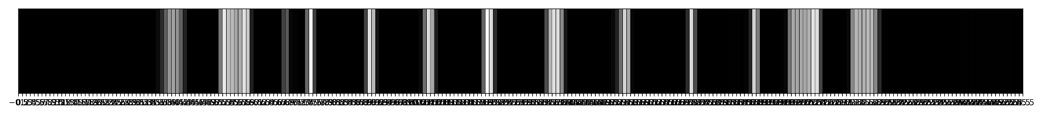
What image is this? Why or why not can you or can you not tell what image it is? Looking at it, it may look like a bar code or something of that sort, but it is not. It is actually a handwritten digit. But even then, which digit is that?
How about now
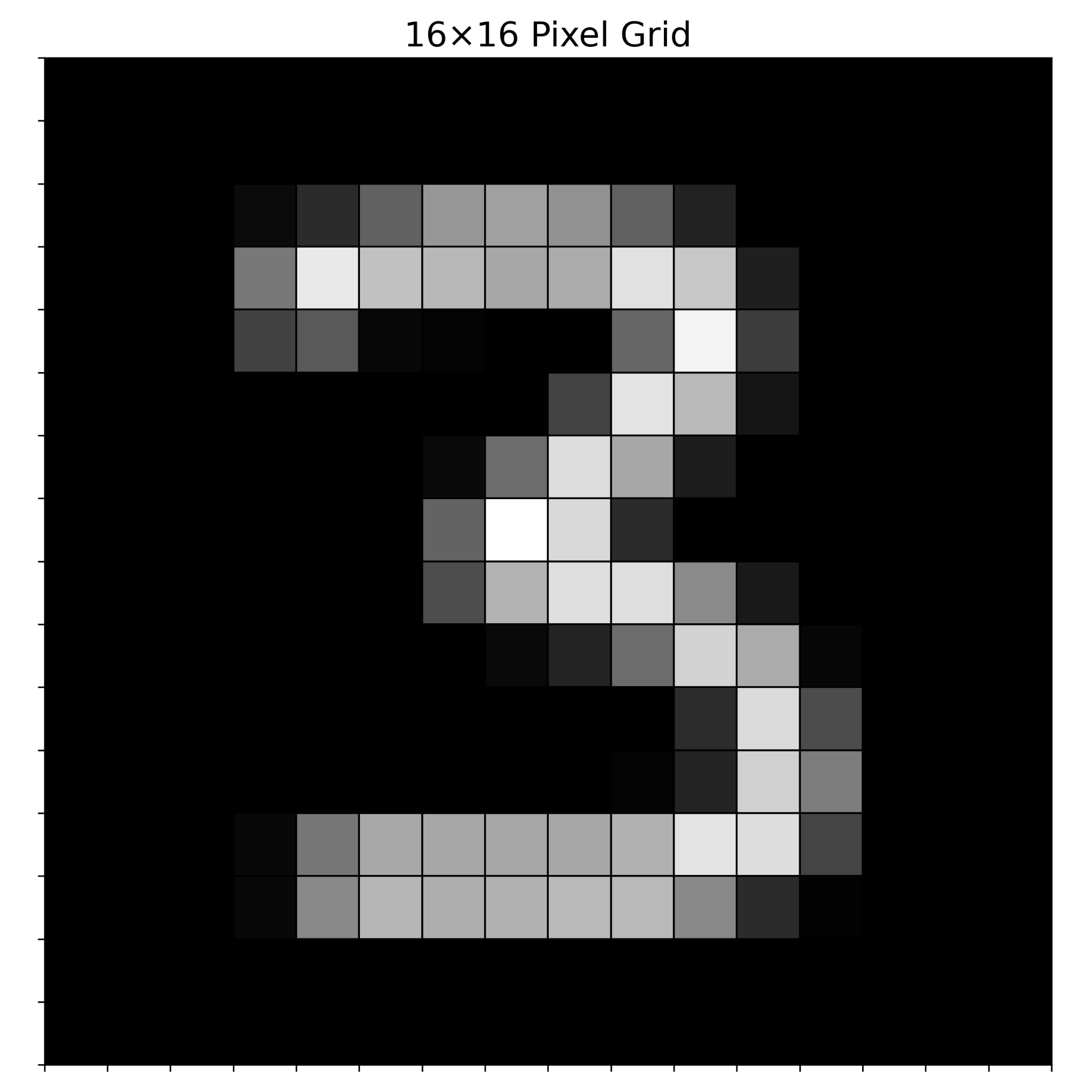
But now, you can clearly see it is a 3.
Now, what was the difference between the first image and the second one? The first image is a linear form of the second one which is a grid. Now, images are usually grids. The grid format contains latent information about an image that makes it unique. These are called features and this concept is called spatial context
When pixel values are flattened into a vector, the neighbourhood relationships between pixels are destroyed. A standard MLP treats pixel 1 and pixel 784 as equally related to pixel 2. Spatially, that is nonsense.
1.2 What Makes a Digit a Digit?
Now, in the above example, what made us conclude that the image is a 3 and not a 6? That is, what makes a 3 a 3 and not an 8 or a 9?
Well, we know that a 3 has edges, and curves. it has some three edges: top, middle, bottom, and two edges on the right. And that makes it a 3.
Now, just as we humans take those points as information and they are enough to tell us that that is a 3 and not an 8, machine learning models need to learn these features.
This not only applies to the handwritten digits example given above. Rather, it generalizes to all other kinds of images. A cat has features like pointy ears, whiskers, tail, etc. A car has four wheels, doors, a windscreen etc. The key idea is that each object in an image has features from which we determine what it is.
Therefore, just as the first example made it difficult to learn what digit is for us, the machine will find it hard also. The first linearized image of a 3 digit is the format in which standard multi-layer perceptrons (MLPs) receive information, which destroys spatial context/information
We want to preserve that spatial information and therefore models must have the image as is.
Then the big question is, how will models learn these features? (edges, curves for this case, and whatever other features are needed for whatever other image there is out there) And in answering that question we must also remember that the images will not come in the exact same format. 1000 different people write '3' differently. A cat may be taken facing east, or west, sitting or standing, it may be brown or black. But in all these cases, the fundamental distinguishing features are the same. How then does a model learn these features?
Before building the solution, we need to understand what we are actually trying to extract. Ask yourself: what makes a 3 a 3, and not an 8 or a 6?
1.3 Kernels: Feature Extractors
This is where the idea of feature extractors come in. Instead of memorizing each digit, we have some special filters that detect these features and extract them, tell if the features are in an image and what they look like. In essence, these extractors can scan the image from start to end, and then extract edges, curves, e.t.c (or whatever other features are there), then based on what features are extracted, where they are extracted etc. the model learns from that and makes a decision.
The mechanism a CNN uses to extract features is called a convolution hence this neural network is called a Convolutional Neural Network. This is performed by the filter, which is a small matrix, called a kernel.
1.3.1 How a Kernel Works
A kernel is a small matrix whose values are learned during training through backpropagation. It operates as follows:
- It is placed over a small patch of the input image
- It asks: does this patch of pixels match the pattern I encode?
- It computes a single output value for that position via element-wise multiplication and summation
- It slides to the next position and repeats
- The full collection of output values forms a new matrix called the feature map
The same kernel - the same learned weights - is applied to every patch of the image. A kernel that detects a horizontal edge will detect it whether that edge appears in the top-left corner or the bottom-right corner. This is called weight sharing, and it is the fundamental reason CNNs are so parameter-efficient compared to MLPs.
1.3.2 Stride and Padding
Two hyperparameters control the mechanics of the convolution:
| Parameter | Definition | Effect |
|---|---|---|
| Stride | The number of pixels the kernel shifts at each step | Larger stride → smaller feature map, faster computation |
| Padding | Extra pixels (usually zeros) added around the image border before convolution | Prevents feature map shrinkage; gives equal attention to edge pixels |
Why padding matters:
Without padding, pixels near the edges of the image are visited by fewer kernel positions than central pixels. The centre gets attended to many more times. Padding fixes both of these:
- It prevents the feature map from shrinking with each convolution
- It gives edge pixels equal weight to centre pixels
1.3.3 Feature Map Size - Deriving the Formula
Let's say you have an image whose dimensions are 5x5, and our kernel is 3x3. We have zero padding, and a stride of 1. What will be the output size of our feature map?
soln:
Lengthwise, the kernel will make
Then add its first position before making those two steps to get:
so the output will be 3 on one dimension, and since the other dimension is identical, the output is:
Now let's say the image is 5x5 and our kernel is 4x4, zero padding, stride of one, what will be the dimensions of the feature map?
hence
Notice then that as the kernel size increases, the feature map size reduces in size. And then also conceptually notice that the edges are traversed less often than pixels at the centre, they don't get as much focus.
Now let's add some padding, and by padding here I mean the number of pixels added to a given edge. so if padding is 2, it is 2 on the left and right margin each as well as on the top and bottom as well.
So, same drill: * input image: 5x5 * kernel: 3x3 * padding: 1 * stride 1
soln
that's
Notice how the dimensionality is maintained across the input and output. That's the purpose that padding serves, it ensures the edges are given as much weight as the centre, and that the size of the feature map does not reduce drastically at each step.
(ask yourself, why are we adding the 1, and why are we dividing by the stride? build intuition for why this is so)
Finally let's build the formula from first principles using the intuition in the examples. Given:
- Input image: $N \times N$
- Kernel: $k \times k$
- Padding: $p$
- Stride: $s$
The padded image becomes $(N + 2p) \times (N + 2p)$. The kernel can be placed at a position as long as it fits entirely within the padded image. The number of positions along one dimension is:
Padding $p = 1$ with a $3 \times 3$ kernel preserves the spatial dimensions of the input exactly. This is so common it has a name: same padding. The output feature map is the same size as the input. The alternative - letting it shrink - is called valid padding.
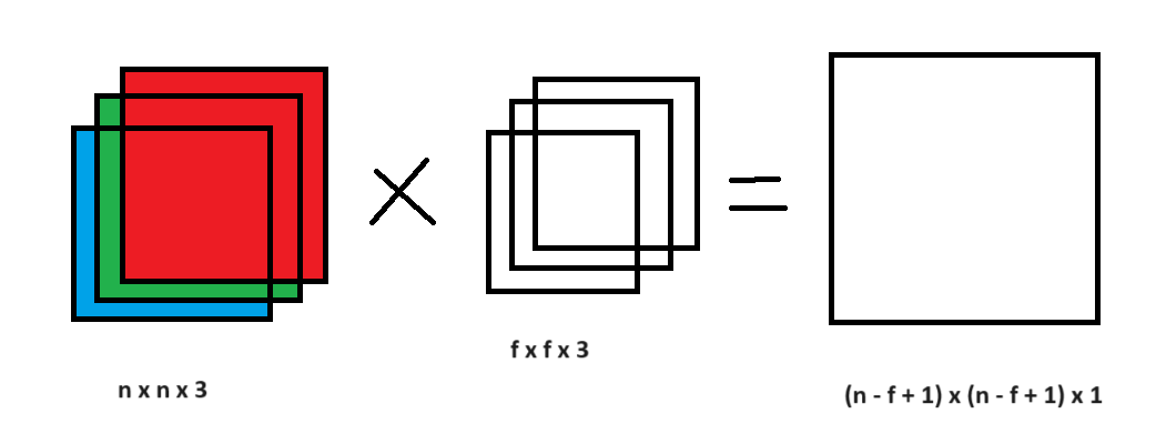
1.3.4 Channels - Extending to Colour Images


So far we have assumed a greyscale image. Such an image is said to have one channel - it is simply shades of one color: gray. But a colour (RGB) image has three channels, that is, it is made up of three primary colors: red, blue, and green


The kernel must now be three-dimensional: $3 \times k \times k$ - one $k \times k$ slice per channel. Each slice is applied to its corresponding colour channel, and the three resulting values are summed to produce a single output value in the feature map.
More generally:
- If the input has $c_{in}$ channels, each kernel is $c_{in} \times k \times k$
- If we want $c_{out}$ different feature maps, we learn $c_{out}$ separate kernels
- Output shape: $c_{out} \times F \times F$
Each of the $c_{out}$ kernels specialises in detecting a different feature. In early layers: edges at various orientations, colour gradients, textures. In deeper layers: combinations of those - corners, shapes, object parts. This hierarchy of features is learned entirely from data.
1.4 Other Layers in a CNN
What we have covered so far under convolution is feature extraction - learned feature extraction because the weights of the kernels are learned during training. The model has other layers, partly that help in the process of feature extraction and another in the actual learning of the task from the extracted features. These layers are: pooling and fully connected layers
1.4.1 Pooling
The function of the pooling layer is to downsample the feature map. Pooling is not learned since it is a fixed mathematical operation. The two common operations are max and average. A filter of a given size, similar in principle to the kernel, but different in operation is used here. The sliding filter, if max will pick the largest in that submatrix, if average will find the average.
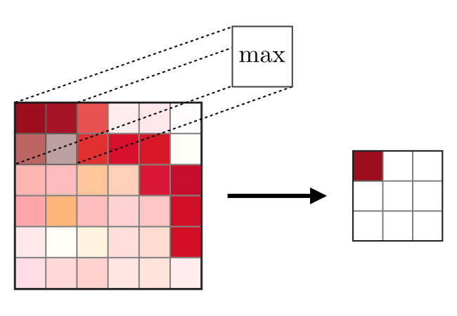
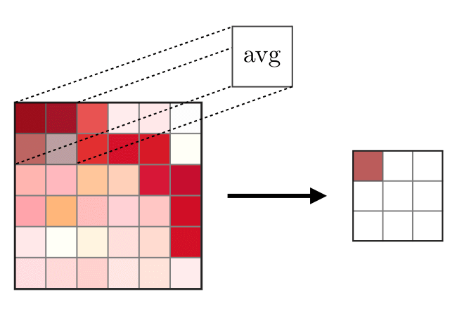
A 2×2 max pooling window with stride 2 reduces each spatial dimension by half.
What pooling achieves:
- Reduces spatial dimensions which cuts computation for subsequent layers.
- Creates slight translation invariance: a feature detected slightly off-centre still produces a strong pooling output
- Retains the most prominent activations (maximum) within each region
Pooling has zero learnable parameters. It is a fixed operation. Only convolution kernels are learned through backpropagation.
1.4.2 Fully Connected Layer
After several rounds of convolution and pooling, the feature maps are flattened into a single vector and passed to one or more standard dense (fully connected) layers.
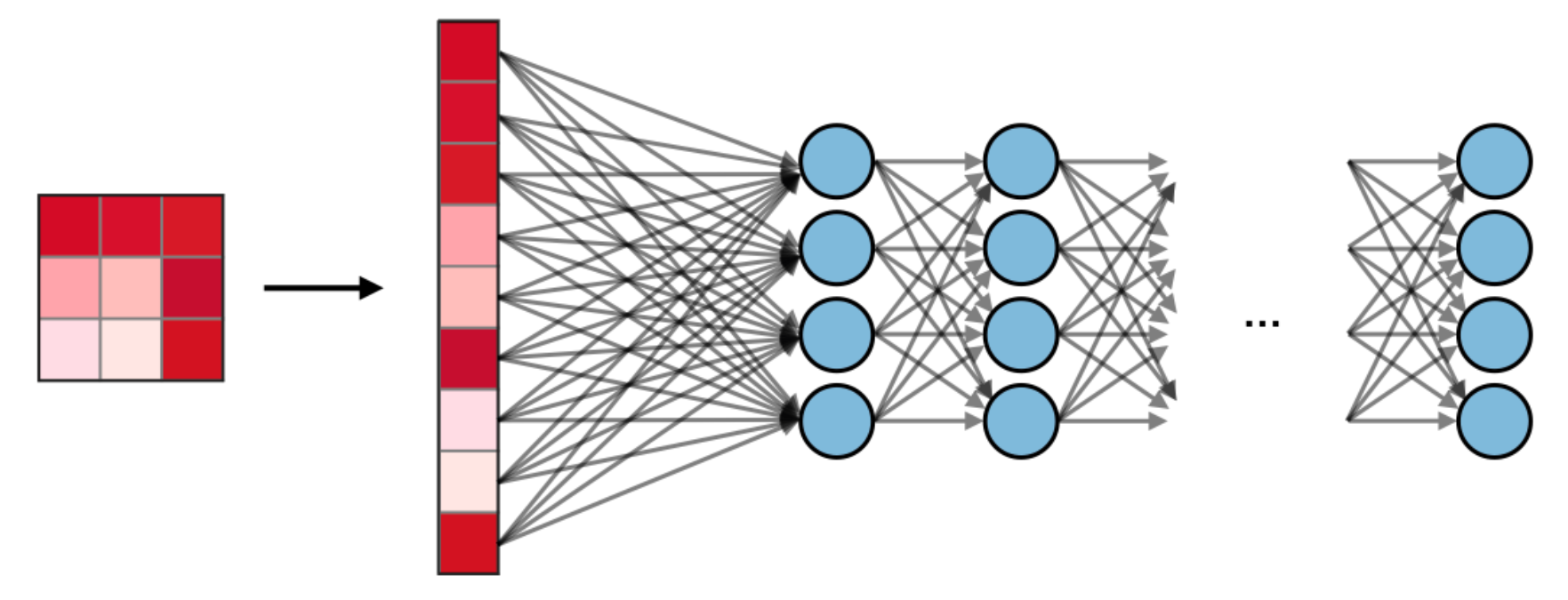
These layers receive a rich set of spatially-extracted features and learn to map them to the final output - for example, a probability distribution over 10 digit classes. This is identical to a standard MLP, but operating on learned features rather than raw pixels.
And this is the special feature of CNNs, that the input to the fully connected layer, is not just the raw pixels transformed into something linear(like the first image), but rather a set of learned features. The fully connected layer now coming after all these convolutions, is doing a fundamentally easier job than an MLP applied to raw pixels.
1.5 The Full CNN Architecture
Full LeNet-style CNN: Input → Conv → Pool → Conv → Pool → Flatten → FC → Output
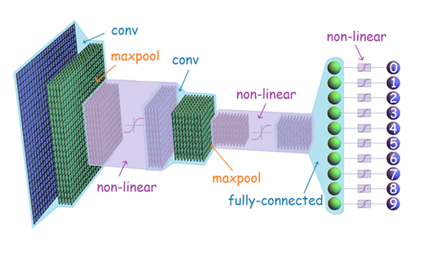
The data flows through a progressive hierarchy:
- Early conv layers detect low-level features, these might look like edges, corners, colour transitions.
- Pooling compresses spatial dimensions while retaining detected features.
- Later conv layers combine low-level features into higher-level representations for example shapes, textures, object parts.
- FC layers use the learned representation to make the final classification decision.
1.6 Parameter Count - CNN vs MLP
Now having looked at a CNN, let us consider how it compares to a standard Multi-Layer Perceptron. Consider the image below:
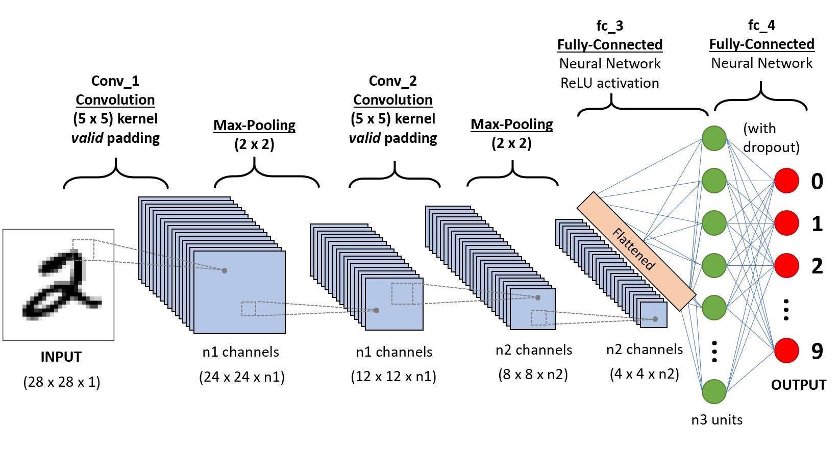
CNN - Conv_1:
Let's say we have 16 kernels
- 16 kernels, each $5 \times 5 \times 1$ (assuming 1 channel, if it was colored, it would be 3)
- input size: $28 \times 28 \times 1$
- output size: $24 \times 24 \times 16$
- Parameters per kernel: $5 \times 5 \times 1 + 1\ (bias) = 26$
- Total Conv_1 parameters: $26 \times 16 = 416$
MLP equivalent:
- Flattened input: $28 \times 28 = 784$ neurons
- Equivalent spatial output: $24 \times 24 \times 16 = 9,216$ neurons
- Fully connected parameters: $(784 + 1) \times 9,216 = 7,234,560$
Now, let's just do the full layer
CNN - Pooling 1:
Now let's apply pooling here
- size: $2 \times 2 \times 1$
- input size: $24 \times 24 \times 16$
- output size: $12 \times 12 \times 16$
- learned parameters: 0
CNN - Conv_2:
Let's say we have 32 kernels for this layer.
- 32 kernels, each $5 \times 5 \times 16$ (Notice now that we have 16 channels, that's because the output of the previous convolution had 16 kernels, hence 16 layers of output.)
- input size: $12 \times 12 \times 16$
- output size: $8 \times 8 \times 32$
- Parameters per kernel: $5 \times 5 \times 16 + 1\ (bias) = 401$
- Total Conv_2 parameters for 32 kernels: $401 \times 32 = 12832$
CNN - Pooling 2:
Now let's apply pooling here
- size: $2 \times 2 \times 1$
- input size: $8 \times 8 \times 32$
- output size: $4 \times 4 \times 32$
- learned parameters: 0
CNN - fc_4:
This layer needs no kernels, it is just a fully connected layer
- input size: $4 \times 4 \times 32$
- hidden_layer (n3 units): 64
- output size: 10
- total parameters:
$$\left( (4 \times 4 \times 32 + 1) \times 64 \right) + \left( (64 + 1) \times 10 \right) = 33,482$$
Full network parameter count:
| Layer | Parameters |
|---|---|
| Conv_1 (5×5×1, 16 kernels) | 416 |
| Pooling 1: | 0 |
| Conv_2 (5×5×16, 32 kernels) | $(5 \times 5 \times 16 + 1) \times 32 = 12,832$ |
| Pooling 2: | 0 |
| fc_4 | $\left( (4 \times 4 \times 32 + 1) \times 64 \right) + \left( (64 + 1) \times 10 \right) = 33,482$ |
| Total | 46,730 |
The CNN achieves better performance on image tasks with 46,730 parameters versus millions for the equivalent MLP. The two reasons are weight sharing (one kernel, many positions) and local connectivity (each kernel only sees a small patch, not all 784 pixels simultaneously). The inductive bias of spatial locality is embedded directly into the architecture.
1.7 CNN Summary
| Property | What CNNs Do |
|---|---|
| Spatial context | Convolution preserves neighbourhood relationships that flattening destroys |
| Weight sharing | One kernel detects one feature type anywhere in the image |
| Hierarchical features | Early layers: edges/textures. Later layers: shapes/parts/objects |
| Parameter efficiency | Orders of magnitude fewer parameters than an equivalent MLP |
| Learned features | Kernels are learned from data via backpropagation - no hand-engineering |
EfficientNet (Tan & Le, 2019) - how to scale CNNs efficiently across depth, width, and resolution simultaneously. MobileNet (Howard et al., 2017) - CNNs under severe resource constraints using depthwise separable convolutions. Both papers are readable and directly extend what was covered in this session.
Part 2 - The Transformer and Global Context
2.1 Motivation - From Space to Sequences
Now, in Part 1 we looked at spatial-sensitive data - images. But what about other forms of data? What other types of data are there that are defined by their characteristics, which in turn informs how they are handled?
The answer is Sequential Data or Temporal Data. This is data that is defined most importantly by order.
Consider the following sentences. Just by changing the position of the word "only," we completely change its meaning:
- "Only she told him that she loved him."
- "She only told him that she loved him."
- "She told only him that she loved him."
- "She told him only that she loved him."
- "She told him that only she loved him."
- "She told him that she only loved him."
- "She told him that she loved only him."
- "She told him that she loved him only."
The exact same words are used in all four sentences, but the sequence dictates the logic. If the spatial context of an image is lost when flattened, the logical context of language is lost when scrambled.
Now, consider another example:
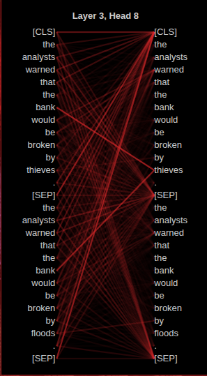
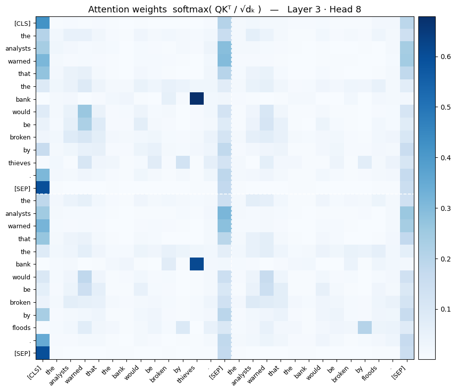
"The analysts warned that the bank would be broken by floods."
The bank here means a riverbank. And the analysts then means environmental analysts.
But what if we change the last word?
"The analysts warned that the bank would be broken by thieves."
Then the bank here means a financial institution. And the analysts then means financial analysts.
This second example shows disambiguation, where the meaning of a word is informed by its context. The word "bank" can be a financial institution or the edge of a river depending entirely on the other words that inform its meaning.
These two concepts - the semantic importance of position and contextual disambiguation - form the principal foundation for why we need architectures built specifically for sequential data.
2.2 Before There Was a Transformer (RNNs and LSTMs)
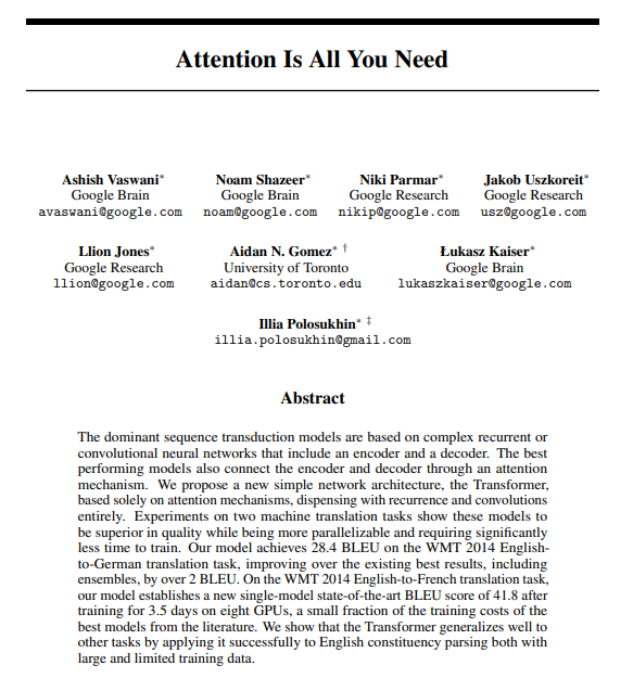
We are primarily going to look at the Transformer architecture, which currently powers ChatGPT, Gemini and the likes. But before the Transformer was invented, there were two primary architectures used for sequential data: Recurrent Neural Networks (RNNs) and Long Short-Term Memory networks (LSTMs).
2.2.1 Recurrent Neural Networks (RNNs)
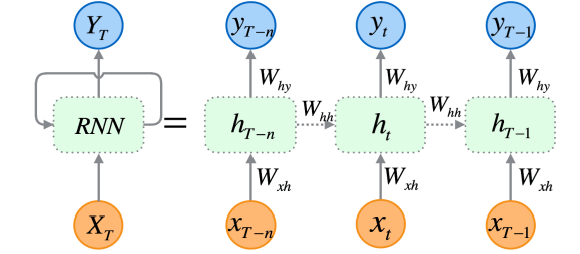
RNNs are like your normal neural networks but with a special feature: recurrence. Each input is indexed temporally. At each step, the network has a hidden state, which acts as a history.
At each time step $t$, the network is fed two things: the current input $x_{t}$ and the previous hidden state $h_{t - 1}$.
Looking at the network spatially, it looks like a single loop, but looking at it temporally (unrolled), it is a chain of steps across time.
For long sequences, standard RNNs suffer from two massive bottlenecks: 1. Memory Compression & Vanishing Gradients: As sequences get longer, earlier context degrades. By the time it reads the 100th word, the 1st word is forgotten. 2. The Sequential Bottleneck: Its sequential nature makes it difficult to parallelize operations. For an input $x_{100}$, we must perform 99 operations sequentially before we can process it.
Long Short-Term Memory (LSTM)
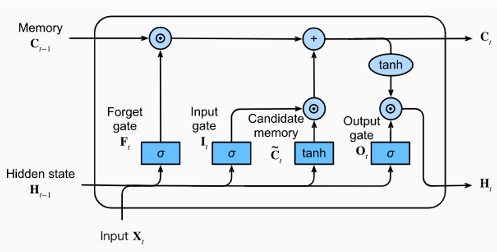
LSTMs were designed to handle the issue of vanishing gradients better than vanilla RNNs. LSTMs introduce gates and cell states. It primarily has three gates: forget, input, output. We will however not go into LSTMs deeply still, but we want to learn how the transformer came to be and why.
However, while designed to handle historical context through a gated "cell state," they still suffer forgetfulness for very long-range sequences. The model eventually loses the broader picture.
More importantly, LSTMs still do not fix the sequential hardware bottleneck. They still read left-to-right, one step at a time.
2.3 Attention: Looking Back
Remember our earlier sentence:
"The analysts warned that the bank would be broken by [floods/thieves]."
What resolves the meaning of "analysts" and "bank"? It is the word after "by" (either floods or thieves). In essence, the word "floods" or "thieves" attends to "bank" and "analysts."
What helped us resolve the meaning of those words 9 and 5 words later? We didn't compress the memory into a single hidden state. Instead, we simply looked back at the exact relevant words. That is attention.
Initially, this Attention technique was added to RNNs and LSTMs to help resolve the long context bottleneck. And it worked - things improved. But there was still an issue: the architecture was still inherently sequential.
What if you get rid of the recurrence entirely?
What if Attention Is All You Need!
2.4 Attention: The Learned Lookup
To understand how Attention works without recurrence, think about a Learned Lookup or a Search Engine (like Google Search). When you want to look up information somewhere, what are the key components?
-
Query (Q): What are you searching for? (e.g., what you type in the search bar).

-
Key (K): How is the available data labelled? (e.g., the SEO tags and titles of web pages).

-
Value (V): What is the actual content?

Attention works in the exact same way, except that the query, key, and value are calculated for each word in the sentence. The Query, Key, and Value are learned matrices. They are represented mathematically as $Q$, $K$, and $V$.
The key twist in a Transformer is that the input itself is typing the queries. The word "bank" acts as a Query (searching for context). The word "floods" acts as a Key. "Bank" matches with that Key, pulls the Value of "floods", and mathematically updates its own meaning.
Below are heat-map matrices of $Q$, $K$, and $V$ extracted from the bert model
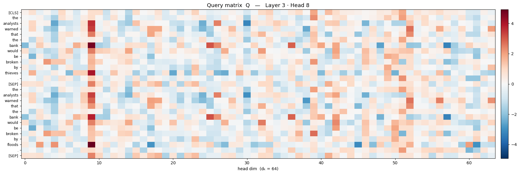
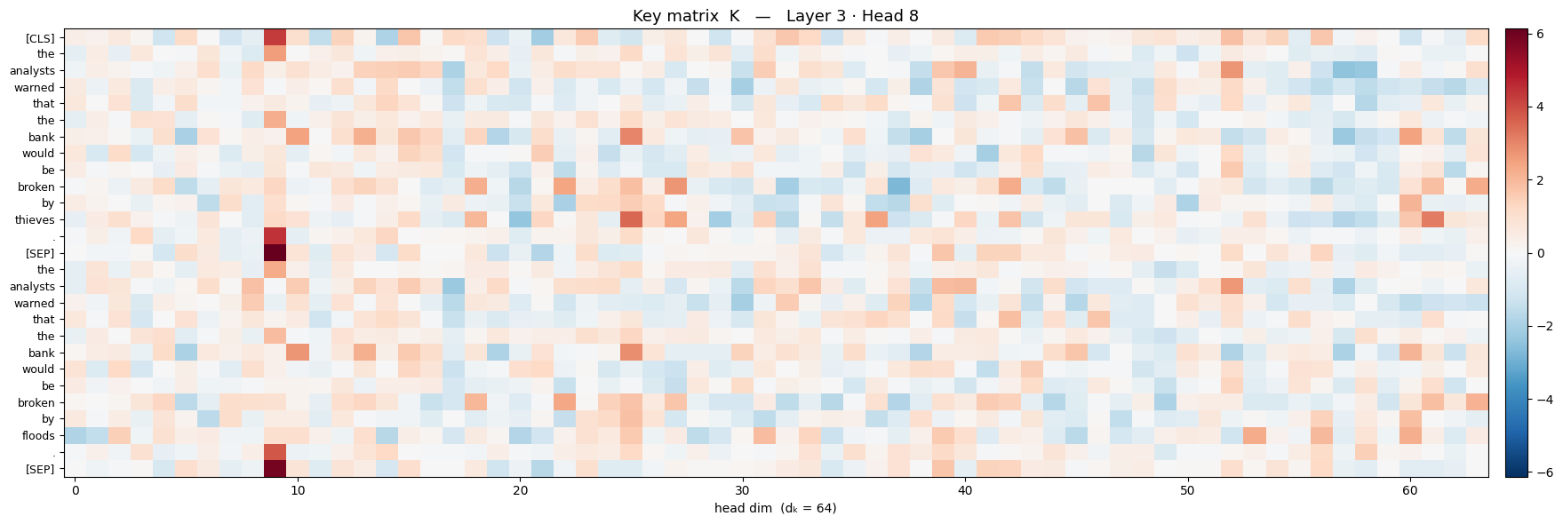
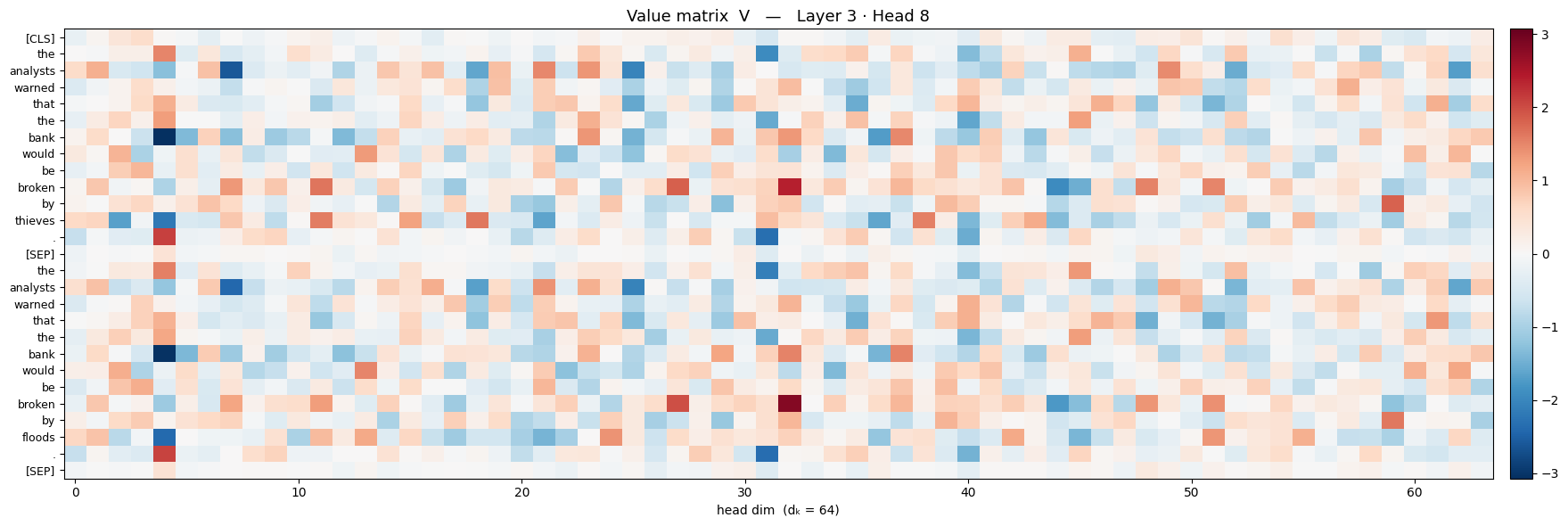
So each word gets it own vector for $q$, $k$ and $v$. Now, the length of each of these is called the embedding dimension, denoted $d_{k}$ . (There is another concept called embedding that we may not cover here, but it is encouraged for the reader to look into it)
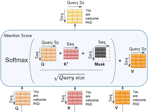
2.5 The Mathematics of Q, K, V Interaction
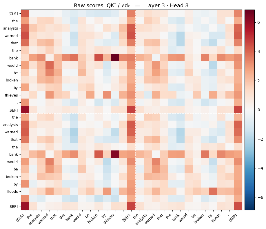
If $Q$, $K$, and $V$ are matrices, how do we get the similarity between two matrices, namely what we are searching for ($Q$) and the labels we are checking against ($K$)?
Remember linear algebra? It is highly useful here (in case you were wondering, as some people do, 'what is the use of all this math', well, here it is 😁). We find the similarity using Cosine Similarity, which in the world of matrices is calculated using the dot product.
However, when we multiply large matrices, the numbers can grow massive. Therefore, we scale the result by dividing by the square root of the embedding dimension ($\sqrt{d_k}$).
Why do we divide by $\sqrt{d_k}$? If we feed massive numbers into a Softmax function, it gets pushed into extreme flat regions where the gradient is exactly 0. Without gradients, the network cannot learn. This scaling stabilizes the values and prevents our gradients from vanishing.
And here is an image of the outputs of the above:
Now, our outputs are all over the place, there is no range, they can be -1000, 34284, 0.23134 etc. So, next we perform a Softmax operation. This scales all the raw similarity scores into percentages that sum up to 1 (e.g., "bank" pays 80% attention to "floods", 15% to "analysts", and 5% to "the").
And now here is the output after softmax:
Finally, we multiply the output of this Softmax with our Value matrix ($V$) to get the actual attention score. This means we are pulling the exact "content" we need, weighted by how relevant it was to our query.
The Final Attention Equation:
And the full flow:
2.6 The Transformer: The Full Architecture
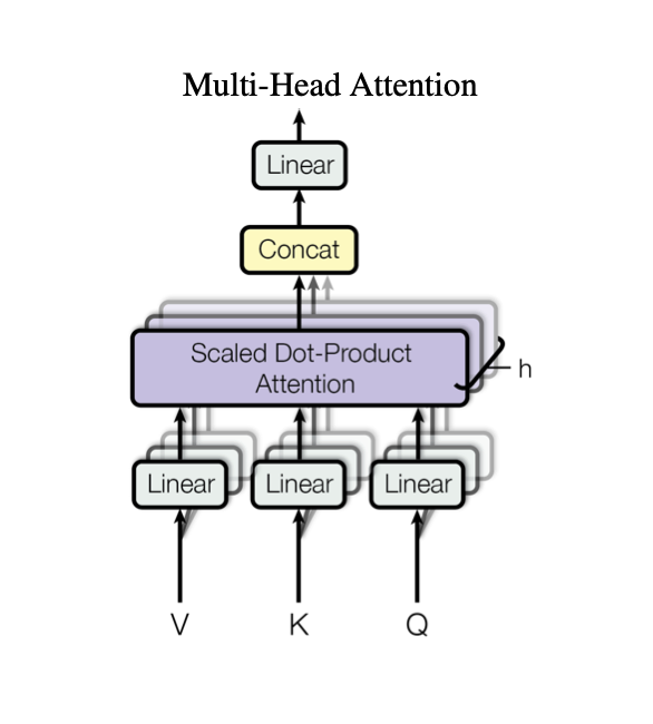
Now, so far we have looked at an example where we have a single set of $Q$, $K$, and $V$, and how they interrelate. That is called Single-Head Attention.
But, instead of a single set of $Q$, $K$, and $V$, we actually use multiple sets simultaneously. This is called Multi-Head Attention. Each "head" learns a different given feature or correlation across the tokens. The results from all the heads are then concatenated and passed through a linear layer.
But how does it all fit together? Here is the full Transformer architecture.
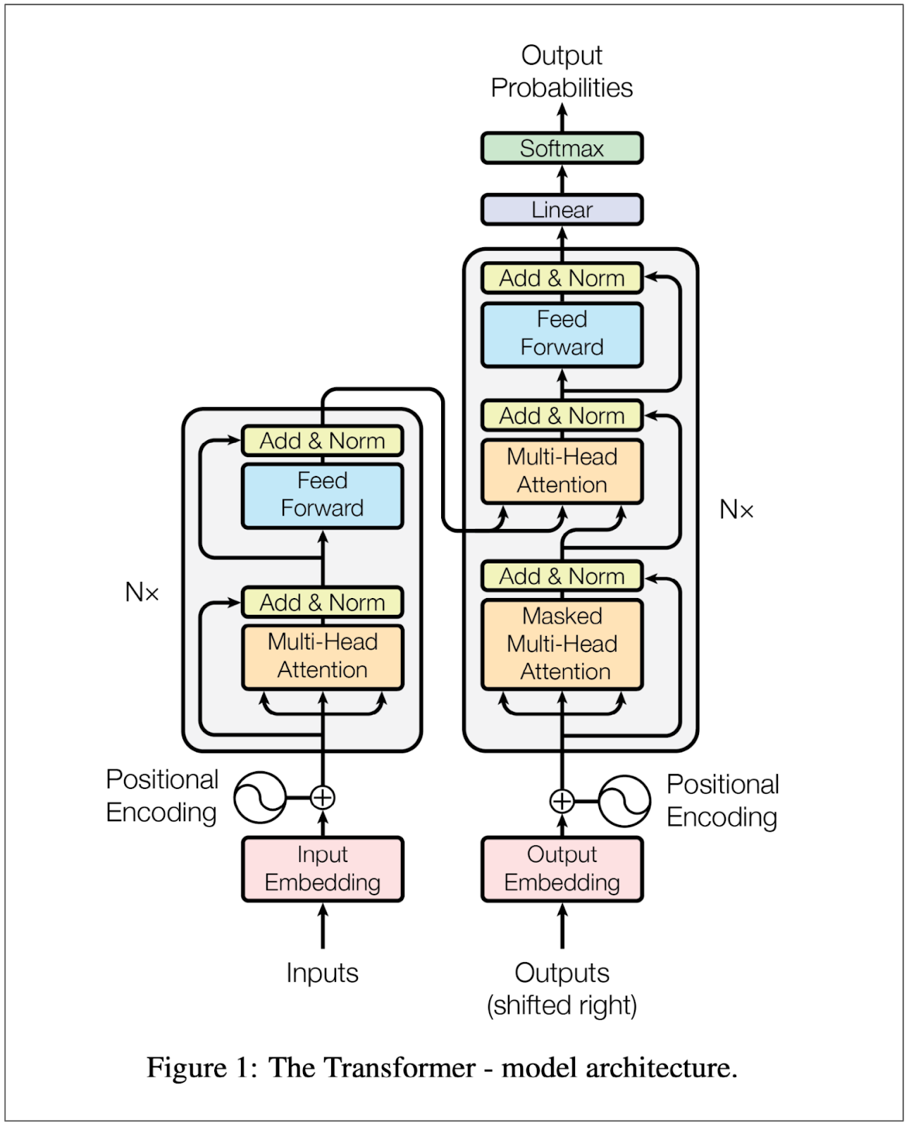
While Multi-Head Attention is the core engine, there are a few other critical components on top of that:
- Notice the positional encoding. Ideally, with attention as discussed so far without positional encoding, the model would read "the boy bit the apple" and "the apple bit the boy" and "the bit apple boy the" all the same since there is no sense of position - the matrices do not inherently encode that, they are order-agnostic. Remember the example of "only" in the sentences above? It would also not know the difference between them. Now, since the whole idea of attention does not have any positional order, we infuse positional encoding through sinusoidal functions and add that to input embeddings.
- Secondly, note the "Add & Norm" layer just after the multihead attention - it simply means we add back the input to the multi-head attention output - this is called residual connection. Its work is to ensure stability during training so that we don't get vanishing gradients. Finally we normalize this combined output.
- Thirdly, Notice the Nx - this means we have N multiple blocks. So the whole Attention+residual connection+feedforward is repeated with each having its input as the output of the previous block. This is what you saw on those screenshots as Layer X alongside the Head Y. So each Layer has Y heads, then we have X layers of such.
- Fourthly, Notice we have two blocks as it were side by side, on the left and on the right. The left one (not due to spatial positioning but due to its architecture) is called the encoder. The right one is called the decoder. Now, the whole essence of the encoder is to capture or, as the word says it, encode the meaning, and content of the input into a standard representative output, called the latent or context vector. The decoder then takes this latent vector and decodes it, that is, uses it to perform the task needed - either translation, generation or whatever the objective of the model is.
- Fifthly, notice the connection between the encoder and decoder. There is an attention block there, leaving aside the masked multihead, the next one. This occurs only once when the two meet, and it is a special kind of attention called cross attention - similar to self attention with the only difference being that the two sequences are not same like in self attention but different.
- Sixthly, notice that the decoder has a special kind of attention so to say, it is called masked multi-head attention. Masking here means, the decoder is not allowed, during training, to see future tokens/words, which it is supposed to generate or else it will just memorize instead of learn, therefore what the decoder sees is masked at each step.
- Finally, remember that attention takes in two sequences - whether similar or different. Now, the size of the attention in terms of the length of the sequence is called context window. This is what you will hear in the sector of LLMs. The larger the context window, the more the transformer can look up at once. When the input exceeds the context window, earlier parts of the sequences are pushed out, it is a FIFO. This explains why in a very long conversation, your chatbot tends to forget things you mentioned very very early on.
2.7 Complexity: RNN/LSTM vs Transformer
Why did the Transformer take over? It is embedded in the math of its complexity. Let $N$ be the length of the sequence.
| Architecture | Total Time Complexity (Operations) | Sequential Steps (Parallel Time) | Space Complexity (Memory) | Meaning / Hardware Behavior |
|---|---|---|---|---|
| RNN / LSTM | $O\left( N \cdot d^{2} \right)$ | $O(N)$ | $O(N \cdot d)$ | Sequential. Step 100 depends entirely on step 99. You cannot parallelize across the sequence length. |
| Transformer | $O\left( N^{2} \cdot d \right)$ | $O(1)$ | $O\left( N^{2} + N \cdot d \right)$ | Parallel. All tokens in a layer can be processed simultaneously, making the architecture highly efficient on GPUs despite the higher total computation. |
Transformers have an (O(1)) sequential step complexity during training because they do not process text step-by-step. Instead of relying on a loop, self-attention allows for massive parallelism across GPUs. This hardware compatibility is what enabled models to scale to billions of parameters using the entire internet as data.
The Transformer pays a heavy price for its parallel training efficiency: a quadratic $O\left( N^{2} \right)$ space and time complexity regarding sequence length. During generation (inference), models use a KV Cache to avoid recomputing past tokens. While this drops the step complexity per token to $O(N \cdot d)$, the memory footprint grows with every word generated.
The maximum sequence length a model is architected to handle is called the Context Window. When a conversation exceeds this window, earlier tokens must be dropped to prevent the GPU from running out of memory (VRAM). This explains why a chatbot will eventually forget things mentioned at the very beginning of an extended, long-form conversation.
2.8 Transformer Summary
| Property | What Transformers Do |
|---|---|
| Global Context | Self-attention calculates relationships between all words simultaneously, ignoring distance |
| Parallelization | Removes the strict sequential bottleneck of recurrence, making training highly efficient on modern accelerators. |
| Context Disambiguation | $Q$, $K$, and $V$ matrices act as a learned search engine, updating a word's meaning based on its surroundings |
| Positional Awareness | Recovers the lost sequential order by stamping sine/cosine waves onto the input embeddings |
Attention Is All You Need (Vaswani et al., 2017) - The foundational paper that introduced this architecture.
BERT (Devlin et al., 2018) - How to use the Encoder stack for bidirectional language understanding.
GPT-3 (Brown et al., 2020) - How scaling the Decoder stack leads to few-shot learning and generation.