Classification Algorithms — Day 2, Session 1

Logistic regression

Logistic regression is a type of regression model that predicts a probability. Logistic regression models have the following characteristics:

The label is categorical. "Logistic regression" usually refers to binary logistic regression — a model that calculates probabilities for labels with two possible values. A less common variant, multinomial logistic regression, calculates probabilities for labels with more than two possible values.
The loss function during training is Log Loss. Multiple Log Loss units can be placed in parallel for labels with more than two possible values.
The model has a linear architecture, not a deep neural network — though the rest of this definition also applies to deep models that predict probabilities for categorical labels.

For example, consider a logistic regression model that calculates the probability of an input email being spam. During inference, suppose the model predicts 0.72. The model is estimating a 72% chance the email is spam, and a 28% chance it is not.

A logistic regression model uses a two-step architecture:

The model generates a raw prediction ($y'$) by applying a linear function of input features.
The model uses that raw prediction as input to a sigmoid function, which converts it to a value between 0 and 1, exclusive.

Like any regression model, logistic regression predicts a number — but that number typically becomes part of a binary classification model: if the predicted number is above the classification threshold, the model predicts the positive class; if it's below, the model predicts the negative class.

The sigmoid function

Many problems require a probability estimate as output. Logistic regression is an extremely efficient mechanism for calculating probabilities. The returned probability can be used either as is (a spam model outputting 0.932 implies a 93.2% probability of spam), or converted to a binary category such as True/False or Spam/Not Spam.

A logistic regression model ensures its output always falls between 0 and 1 by passing its raw prediction through the standard logistic function — better known as the sigmoid function ("sigmoid" meaning "s-shaped"):

$$f(x) = \frac{1}{1 + e^{-x}}$$

f(x) is the output of the sigmoid function.
e is Euler's number: a mathematical constant ≈ 2.71828.
x is the input to the sigmoid function.

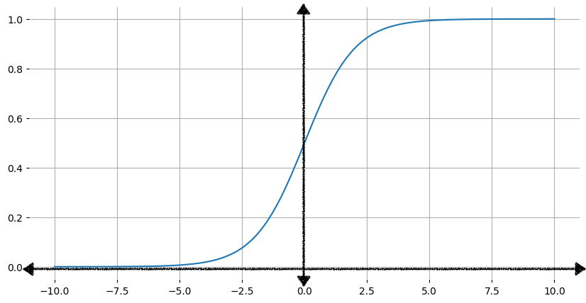
Graph of the sigmoid function, an s-shaped curve bounded between 0 and 1 — **Figure 1.** Graph of the sigmoid function. The curve approaches 0 as x values decrease toward negative infinity, and 1 as x values increase toward infinity.

As the input x increases, the sigmoid's output approaches but never reaches 1. As the input decreases, the output approaches but never reaches 0.

Transforming linear output using the sigmoid function

The linear component of a logistic regression model is:

$$z = b + w_1x_1 + w_2x_2 + \dots + w_nx_n$$

z is the output of the linear equation, also called the log odds.
b is the bias.
The w values are the model's learned weights.
The x values are the feature values for a particular example.

To obtain the logistic regression prediction, z is passed to the sigmoid function, yielding a probability between 0 and 1:

$$y' = \frac{1}{1 + e^{-z}}$$

Side-by-side graphs: a straight linear function on the left transformed into an s-shaped sigmoid curve on the right — **Figure 2.** Left: graph of the linear function z = 2x + 5, with three points highlighted. Right: the sigmoid curve, with the same three points highlighted after being transformed by the sigmoid function.

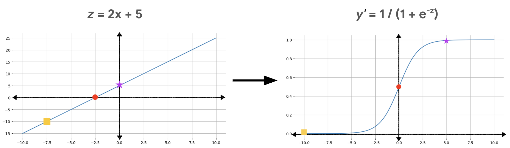
The linear equation can output very big or very small values of z, but the sigmoid's output, y', is always between 0 and 1, exclusive. For example, a z value of −10 maps to a y' value of just 0.00004.

Quiz

A logistic regression model with three features has the following bias and weights:

$b = 1$
$w_1 = 2$
$w_2 = -1$
$w_3 = 5$

Given the input values $x_1 = 0$, $x_2 = 10$, $x_3 = 2$ — answer the following:

What is the value of z for these input values?
What is the logistic regression prediction for these input values?

Loss & regularization

Logistic regression models are trained using the same process as linear regression models, with two key distinctions: they use Log Loss instead of squared loss, and applying regularization is critical to prevent overfitting.

Log Loss

Squared loss works well for a linear model, where the rate of change of the output is constant. But the rate of change of a logistic regression model is not constant — the sigmoid curve is s-shaped rather than linear. When the log-odds (z) value is close to 0, small increases in z cause much larger changes in y than when z is a large positive or negative number.

If squared loss were used, the closer the output got to 0 or 1, the more memory would be needed to preserve the precision required to track the differences. Instead, logistic regression uses Log Loss:

$$\text{Log Loss} = -\frac{1}{N}\sum_{i=1}^{N}\left[y_i \log(y_i') + (1 - y_i)\log(1 - y_i')\right]$$

N is the number of labeled examples in the dataset.
i is the index of an example in the dataset.
y_i is the label for the ith example — either 0 or 1.
y_i' is the model's prediction for the ith example, given its features.

Regularization in logistic regression

Without regularization, the asymptotic nature of logistic regression would keep driving loss toward 0 in cases where the model has a large number of features. Most logistic regression models use one of two strategies to control complexity:

L2 regularization.
Early stopping: limiting training steps to halt training while loss is still decreasing.

Classification is the task of predicting which of a set of classes (categories) an example belongs to.

Binary classification

Binary classification predicts one of two mutually exclusive classes: the positive class and the negative class. For example:

A model that determines whether an email is spam (positive) or not spam (negative).
A model that evaluates medical symptoms to determine whether a person has a particular disease (positive) or doesn't (negative).

Thresholds & the confusion matrix

Say you have a logistic regression model for spam detection that predicts a value between 0 and 1, representing the probability that a given email is spam. To deploy this model, you need to convert its raw numerical output into one of two categories: "spam" or "not spam." You do this by choosing a classification threshold. Examples above the threshold are assigned to the positive class; examples below are assigned to the negative class.

Suppose the model scores one email at 0.99 and another at 0.51. At a threshold of 0.5, both are classified as spam. At a threshold of 0.95, only the 0.99 email is classified as spam. 0.5 might seem intuitive, but it's not a good default if the cost of one type of wrong classification is greater than the other, or if the classes are imbalanced — labelling anything ≥50% likely as spam produces poor results when only 0.01% of emails actually are spam.

Confusion matrix

The probability score is not reality, or ground truth. There are four possible outcomes for each output of a binary classifier — laid out below as a confusion matrix, with ground truth as columns and the model's prediction as rows.

Confusion matrix — spam classifier example
	Actual positive	Actual negative
Predicted positive	True positive (TP): a spam email correctly classified as spam — automatically sent to the spam folder.	False positive (FP): a legitimate email misclassified as spam, and sent to the spam folder.
Predicted negative	False negative (FN): a spam email misclassified as not-spam, that makes its way into the inbox.	True negative (TN): a legitimate email correctly classified as not-spam, sent directly to the inbox.

Each row totals all predicted positives (TP + FP) or all predicted negatives (FN + TN), regardless of validity. Each column totals all real positives (TP + FN) or all real negatives (FP + TN), regardless of model classification.

When the total of actual positives isn't close to the total of actual negatives, the dataset is imbalanced — for example, thousands of cloud photos where the rare cloud type you care about appears only a handful of times.

Accuracy, recall, precision & F1

TP/FP/TN/FN feed several evaluation metrics. Which metric matters most depends on the model, the task, the cost of different misclassifications, and whether the dataset is balanced. All metrics below are calculated at a single fixed threshold, and change as the threshold changes.

Accuracy

Accuracy is the proportion of all classifications that were correct:

$$\text{Accuracy} = \frac{TP + TN}{TP + TN + FP + FN}$$

A perfect model has zero false positives and zero false negatives — accuracy of 1.0. On a balanced dataset, accuracy is a reasonable coarse-grained measure, which is why it's often the default metric for generic tasks. But on an imbalanced dataset, or where one kind of mistake is costlier than the other (the case in most real-world applications), it's better to optimize for one of the other metrics. On a heavily imbalanced dataset where the positive class appears just 1% of the time, a model that always predicts negative scores 99% accuracy despite being useless.

Recall, or true positive rate

The true positive rate (TPR), or recall, is the proportion of all actual positives correctly classified as positive:

$$\text{Recall (TPR)} = \frac{TP}{TP + FN}$$

In the spam example, recall measures the fraction of spam emails correctly caught — hence its other name, probability of detection. A perfect model has zero false negatives and a recall of 1.0. In an imbalanced dataset with very few actual positives, recall is often more meaningful than accuracy — for disease prediction, a false negative typically has more serious consequences than a false positive.

False positive rate

The false positive rate (FPR), or probability of false alarm, is the proportion of actual negatives incorrectly classified as positive:

$$FPR = \frac{FP}{FP + TN}$$

A perfect model has zero false positives — FPR of 0.0. FPR is generally more informative than accuracy on imbalanced data, but grows volatile when actual negatives are very few — with only four actual negatives, a single misclassification jumps FPR to 25%.

Precision

Precision is the proportion of all positive classifications that are actually positive:

$$\text{Precision} = \frac{TP}{TP + FP}$$

In the spam example, precision measures the fraction of emails classified as spam that actually were spam. A hypothetical perfect model has zero false positives — precision of 1.0. Precision improves as false positives decrease, recall improves as false negatives decrease — and since raising the classification threshold tends to trade one for the other, precision and recall often move in opposite directions.

Choice of metric and tradeoffs

Metric guidance
Metric	Guidance
Accuracy	Use as a rough indicator of training progress on balanced datasets; combine with other metrics for real evaluation. Avoid on imbalanced datasets.
Recall (TPR)	Use when false negatives are more expensive than false positives.
False positive rate	Use when false positives are more expensive than false negatives.
Precision	Use when it's very important for positive predictions to be accurate.

F1 score

The F1 score is the harmonic mean of precision and recall:

$$F1 = 2 \times \frac{\text{Precision} \times \text{Recall}} {\text{Precision} + \text{Recall}} = \frac{2TP}{2TP + FP + FN}$$

This metric balances precision and recall, and is preferable to accuracy for class-imbalanced datasets. When precision and recall are both 1.0, F1 is also 1.0. When precision and recall are close, F1 sits close to their value; when they're far apart, F1 skews toward whichever is worse.

Quiz

A model outputs 5 TP, 6 TN, 3 FP, and 2 FN. Calculate the recall.
A model outputs 3 TP, 4 TN, 2 FP, and 1 FN. Calculate the precision.

ROC and AUC

Receiver-operating characteristic curve (ROC)

The ROC curve is a visual representation of model performance across every threshold — the name is a holdover from WWII radar detection. It's drawn by calculating the true positive rate (TPR) and false positive rate (FPR) at every possible threshold, then graphing TPR over FPR.

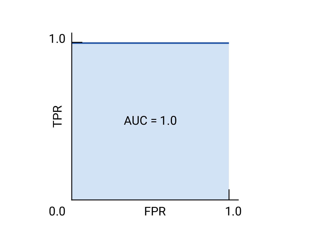
ROC curve of a hypothetical perfect model, forming a square with a corner at true positive rate 1 and false positive rate 0 — **Figure 1.** ROC and AUC of a hypothetical perfect model — one that, at some threshold, achieves a TPR of 1.0 and an FPR of 0.0.

Area under the curve (AUC)

The area under the ROC curve (AUC) represents the probability that the model, given a randomly chosen positive and negative example, will rank the positive higher than the negative. The perfect model above — a square with sides of length 1 — has an AUC of 1.0: a 100% probability of correctly ranking a random positive example above a random negative one.

A horizontal spread of predicted scores for a binary classification model, showing squares (positive examples) and circles (negative examples) — **Figure 2.** A spread of predictions for a binary classification model. AUC is the chance a randomly chosen square (positive) is positioned to the right of a randomly chosen circle (negative).

Prediction bias

Calculating prediction bias is a quick check that can flag issues with the model or training data early on. Prediction bias is the difference between the mean of a model's predictions and the mean of the ground-truth labels. A model trained on a dataset where 5% of emails are spam should predict, on average, that 5% of emails are spam. If it does, the model has zero prediction bias — though it may still have other problems.

If the model instead predicts spam 50% of the time, something is wrong with the training data, the applied dataset, or the model itself. Prediction bias can be caused by:

Biases or noise in the data, including biased sampling for the training set.
Too-strong regularization, which oversimplifies the model and loses necessary complexity.
Bugs in the model training pipeline.
A feature set that's insufficient for the task.

Multi-class classification

Multi-class classification extends binary classification to more than two classes. If each example belongs to exactly one class, the problem can be decomposed into a series of binary classification problems — one class against all the others, repeated for each original class.

For example, classifying examples with labels A, B, and C could become two binary classifiers: first, A+B versus C; then, among examples labelled A+B, A versus B. A handwriting classifier that decides which digit (0–9) an image represents is a classic multi-class problem.

If class membership isn't exclusive — an example can belong to multiple classes at once — that's a multi-label classification problem instead.

References

Google Machine Learning Crash Course ↗