1. Decision Trees
1.1 Motivation
Recap on logistic regression: learns a hyperplane as a decision boundary, to separate two classes.
But what about?
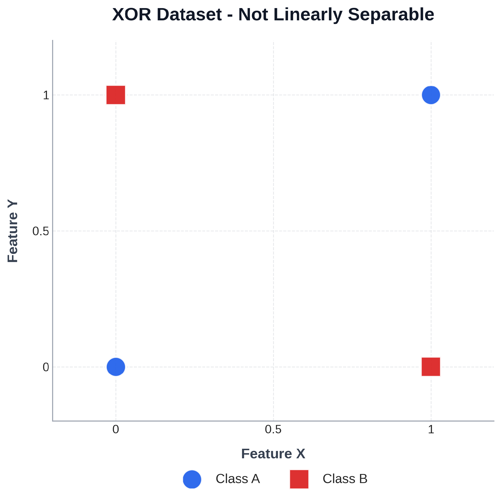
Is this problem linearly separable? No, it cannot be linearly separable.
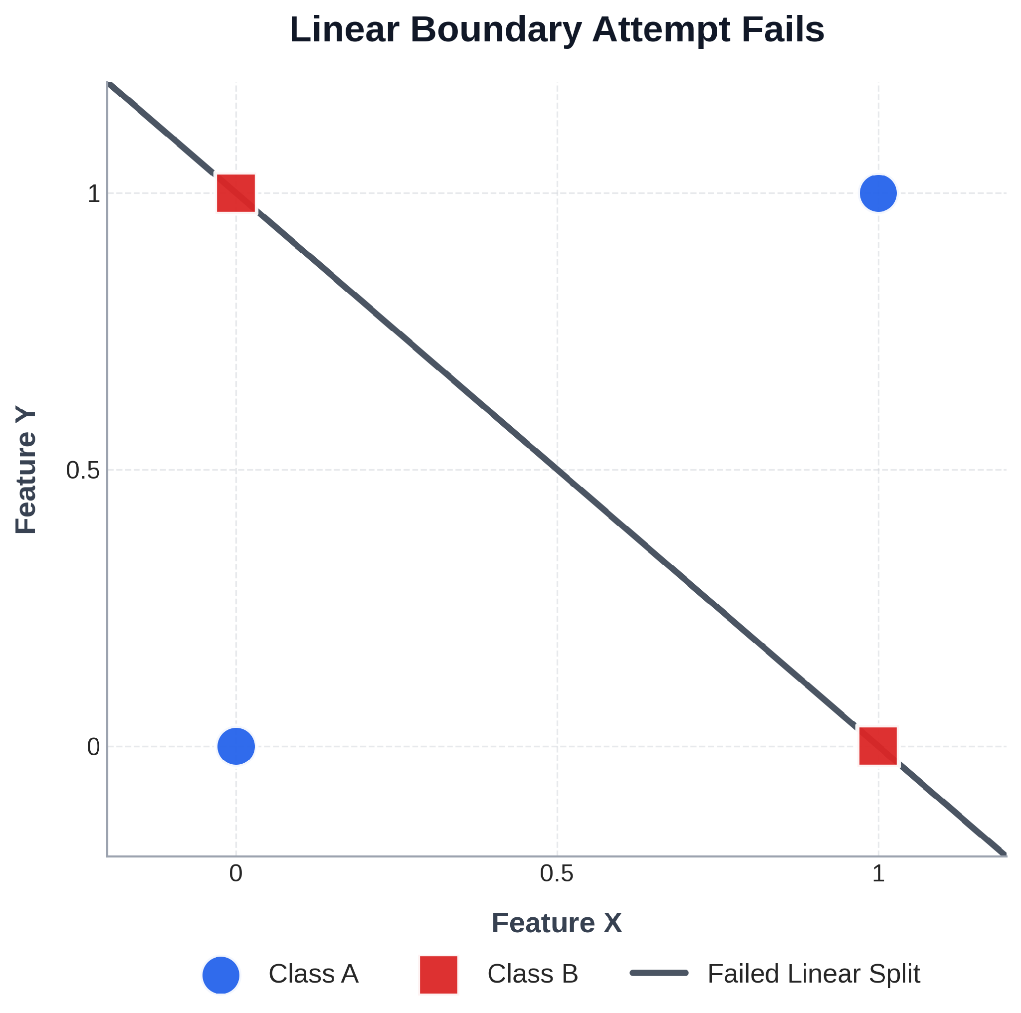
Now, there are other means of solving this. We may not get into it, but for now this will serve as a motivation for what we are going to be learning today: Decision trees and related concepts.
But is it still possible to classify this data, even in a non-linear fashion? Yes. How?
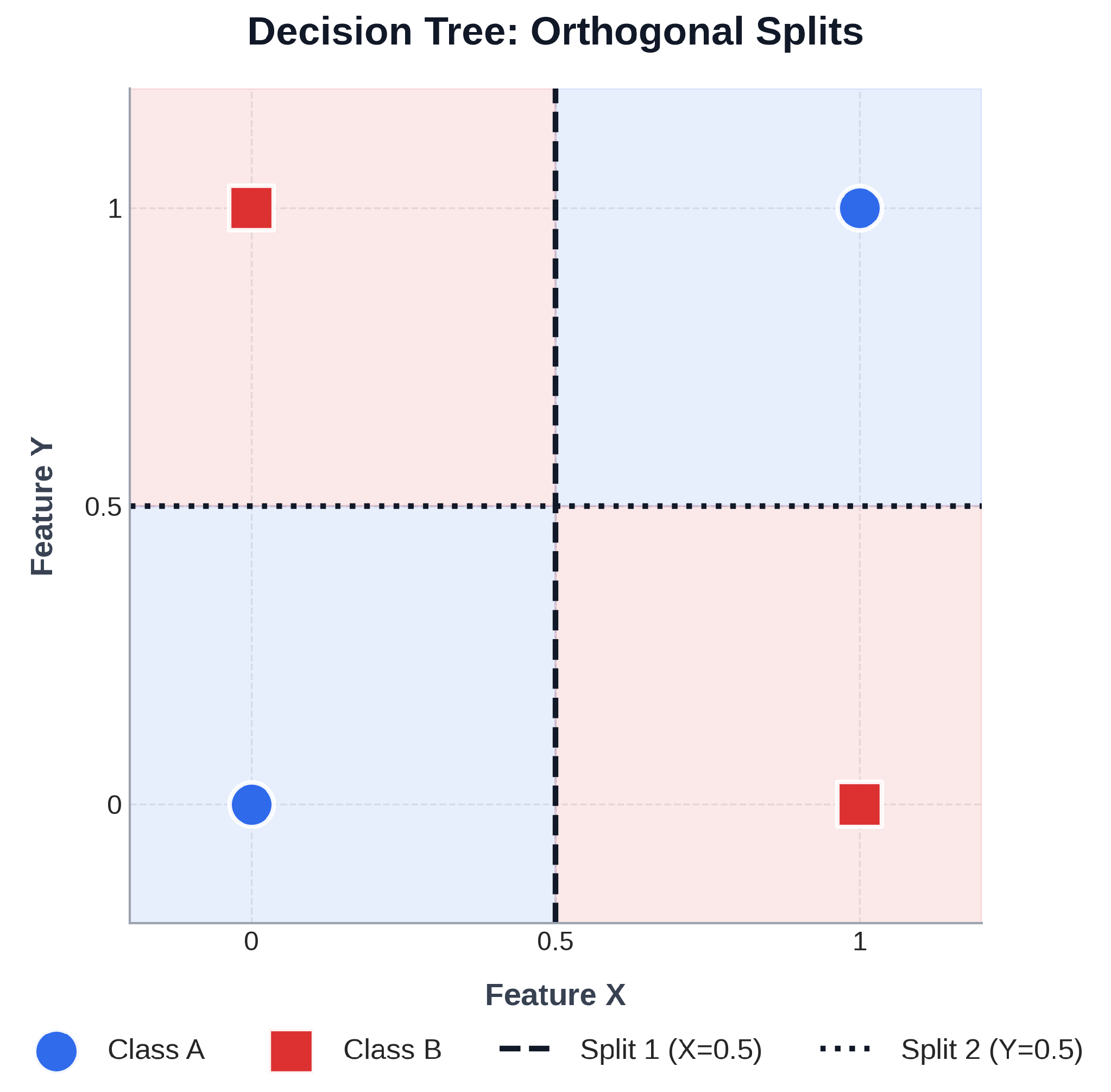
We can have two perpendicular lines that divide into four regions with each class having two regions.
Now, how was this achieved practically? These lines can be viewed as decision boundaries — as points of decision, answers to questions.
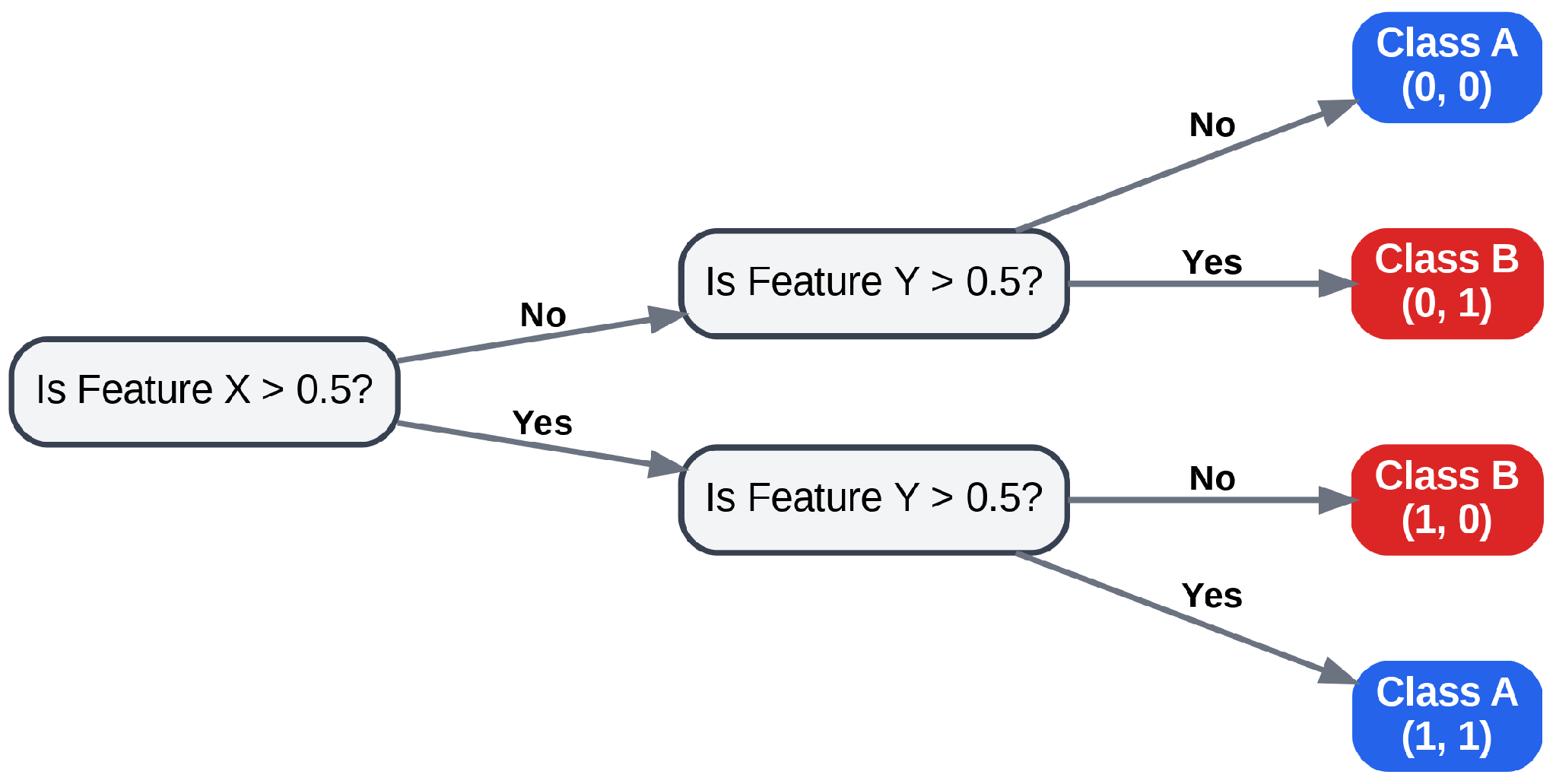
The above example is actually an XOR. You will realize that the two classes correspond to XOR, just a side note worth mentioning.
1.2 Anatomy of a Decision tree.
That is how the tree looks like. Notice at each step we have a question, and possible answers. Each node is a question, each edge is a potential answer, and each leaf is a decision. That is basically how decision trees operate. Now, the root node is the first question, and the depth of a tree is the number of steps or questions (i.e. branches) between the root node and the decision in the leaf node. Depth controls the tree's complexity.
But the big question is, what is the best question to ask at each step? All questions are not equal. There are some questions, based on whatever context, whose answers carry more weighty significance and give you more info compared to others. Therefore what we are going to spend a significant amount of time in this session is learning to ask the best questions at each step."
1.3 What makes a good split?
To motivate and guide us through this section, we will use a simple dataset.
| Temperature | Raining? | Went for a Run? |
|---|---|---|
| Hot | No | No |
| Hot | No | No |
| Cold | No | Yes |
| Cold | Yes | No |
| Hot | Yes | No |
| Cold | No | Yes |
The big question is, should we go for a run given temperature and rain conditions and our history of going for a run?
Which question should we ask first? Remember the target variable is whether we went for a run or not. Notice: we are studying the intuition behind building the tree, we are not focusing on the output of the tree. What we need is step by step construction of the tree.
So, what are the two questions: 1. Is it hot or cold? 2. Is it raining or not?
Okay, now that we have the two possible questions for our scenario, let us ask ourselves, what makes a good question? A good question always splits the data in a way that makes things clearer, more predictable — that is, produces classes that are purer, where most or all examples in a group belong to one class. A bad question produces classes that are mixed, unpredictable and does not help improve the distinction of the classes. The measure of how mixed a group is, how unpredictable, is called entropy.
So, before we look into which of these questions is better, we must look at entropy, which is the measure that determines that.
1.4 Entropy
Suppose we wish to define a mathematical function that measures the unpredictability or surprise of observing an event. What would it look like? What would be its characteristics? What would it be?
Let's say we have a bag with 100 red marbles and 0 blue marble. What is the probability of picking a red marble? It is 1.0. Now, how surprised would you be if you picked a red marble? Not at all, There is no surprise at all if you picked a red marble, that is because it is very predictable, it is fully predictable. Therefore the uncertainty before drawing is zero. Observing the draw gives us zero information because the outcome was already certain.
This is the first characteristic of such a function
and consequently also
This first characteristic also tells us that as probability increases, surprise, unpredictability, and also information decreases.
Now another case: suppose I first tell you the outcome of a coin toss, and then independently tell you the outcome of a die roll. The total information you have gained should be the information from the first observation plus the information from the second. Since the events are independent, neither observation changes the surprise associated with the other.
If we label the two events as $X$ and $Y$, then the probability of both occurring is
And thus:
Now, based on the above characteristics and formulations, which function comes to mind?
logarithm: $\log$,
Why? Logarithms convert multiplication to addition.
but, letting $x = P(X)$ w.l.o.g,
So, what do we do to fit this? We add a negative. Thus
Therefore, our function to characterize unpredictability is:
But this is for a single incident. To cater for all occurrences, we must weight this measure with the probability. This is the expected value — the average surprise over all possible outcomes. Now the $x$ variable is the probability $P(X)$. so our formula would boil down to:
But this is for one occurrence, the probability that it is $A$. What we want is the overall unpredictability of the whole set. How do we find the overall average of different probabilities in statistics? We calculate the expected value. We multiply each outcome's surprise by its probability of happening, and add them all up.
This is the formula for entropy, which is labelled as $H(X)$, thus:
Let's validate this on the marbles case:
case 1:
case 2:
By convention
Since
1.5 Information Gain
Now, step by step, the decision tree uses this notion of entropy to make a decision at each step. But how does it do this? It aims to reduce unpredictability, uncertainty, or rather, gain as much information as possible. To do that, it calculates entropy before and after a probable step and then gets the difference. But the entropy after is weighted.
So, let's say entropy at starting point is $H(S)$. We calculate the weighted sum of each entropy and get the difference. Let $IG$ be information gain, and $A$ be the feature then:
where $\frac{|S_{v}|}{|S|}$ is a fraction of the data that went down to the path where $A = v$.
The fraction $\frac{|S_{v}|}{|S|}$ ensures larger child groups carry more weight — a split that produces one large pure group and one tiny impure group is still a good split overall.
1.6 Back to our example
| Temperature | Raining? | Went for a Run? |
|---|---|---|
| Hot | No | No |
| Hot | No | No |
| Cold | No | Yes |
| Cold | Yes | No |
| Hot | Yes | No |
| Cold | No | Yes |
First step, let us get the baseline entropy $H(S)$
Now, we have two options. We start with the first question
Temperature: Is it hot or cold? If we split the table based on temperature, we get two children groups:
1. Cold Group (3 mornings): 2 Runs (Yes), 1 No Run (No).
2. Hot Group (3 mornings):
Now, we calculate the weighted average of these new entropies.
Information gain for temperature
Now, let's see the second question.
Rain: Is it raining?
1. Rain = Yes (2 Mornings): 0 Runs (Yes), 2 No Runs(No). This group is perfectly pure, so:
2. Rain = No (4 mornings): 2 Runs (Yes), 2 No Runs (No). This is a perfect 50, 50 split:
Now, calculating the weighted average
Information gain for rain:
So which is the better question? Splitting on temperature or splitting on rain? Splitting on temperature gives us an information gain of 0.459 and splitting on rain gives us a gain of 0.251. Therefore the question "Is it hot or cold?" clears way more uncertainty than "Is it raining or not?" This is the math that the tree does at every step recursively, until the desired result is achieved.
We have so far discussed entropy as the primary impurity measure used to choose splits. However, in implementation (like scikit-learn), a different impurity approximator called the Gini index is often used by default.
While entropy measures "information surprise," Gini measures the probability of misclassification. If you randomly pull a sample from a node and randomly label it according to the distribution of that node, what is the chance you get it wrong?
The formula is: $Gini = 1 - p_{i}^{2}$
Why use it?
Entropy requires calculating logarithms, which are computationally expensive. Gini only requires squaring numbers, making it slightly faster to compute across massive datasets. In practice, they produce nearly identical trees, but Gini is preferred for execution speed.
But how do we know the desired result? How do we know when to stop?
1.7 Overfitting and Regularization
It may at first look intuitive to let the tree run until every single leaf node is perfectly pure i.e. $H = 0$. But this brings issues. While it may achieve perfect training accuracy, it will also have learned noise and outliers — overfitting. When presented with new data that it was not trained on, it will fail.
Now, how can we stop this? There are a few regularization constraints, which are hyperparameters, that we can impose on the algorithm when building the tree.
| Hyperparameter | What it does |
|---|---|
max_depth |
Hard limit on tree depth — the primary dial |
min_samples_split |
Minimum examples required to split a node |
min_samples_leaf |
Minimum examples required in a leaf |
min_impurity_decrease |
Minimum gain required for a split to proceed |
Now, just as the tree can overfit if it is too deep, it can also underfit if too shallow. So there must be a balance between the two extremes to get a proper balance. The table below shows the relation between depth, bias, and variance.
| Tree Depth | Bias | Variance | Effect |
|---|---|---|---|
| Very shallow | High | Low | Underfits — too simple to capture patterns |
| Moderate | Balanced | Balanced | Generalises well |
| Fully grown | Low | High | Overfits — memorises training noise |
Therefore, depth is a key complexity dial for a decision tree. When it is high, complexity is also high and vice versa. The tree generalizes well when the right depth is attained. Thorough cross-validation helps in finding the right depth.
1.8 Summary
| Property | What Decision Trees Do |
|---|---|
| Non-linear boundaries | Orthogonal splits carve the feature space into rectangular regions |
| Interpretability | Every prediction can be traced root to leaf and explained in plain language |
| No feature scaling | Splits are threshold-based, not distance-based — normalisation is not needed |
| Handles mixed data | Works natively with both numerical and categorical features |
| High variance | Small changes in training data can produce a completely different tree |
CART — Classification and Regression Trees (Breiman, Friedman, Olshen & Stone, 1984) — the foundational algorithm behind scikit-learn's implementation. Introduced binary recursive partitioning and cost-complexity pruning. Chapter 3 covers tree growing and pruning at an accessible level.
C4.5 (Quinlan, 1993) — the algorithm that extended CART to handle continuous features, missing values, and post-pruning natively. Understanding it deepens intuition for the design decisions sklearn makes under the hood.
StatQuest: Decision Trees (Josh Starmer, YouTube) — the clearest visual walkthrough of entropy, information gain, and tree building available. Watch before the practical session.
2. Ensemble Methods
2.1 Introduction
Now that we have looked at trees, what is a probable demerit of a decision tree? and why?
Instability. A single tree is highly sensitive to even small variations making it unstable. This is where we have to look for means of giving stability to a decision tree, or rather the technique we have looked at so far. And how do we do that? Ensemble methods
Now, what are ensemble methods? The key idea is that you don't just have one tree, but a group of trees together where the decision is arrived at as an aggregate of all the decisions of the all trees. The only condition here is that the errors of the trees be uncorrelated because otherwise they will not balance each other out. In this case aggregation does not help. When they are uncorrelated, the weaknesses and failures of one tree are covered up by the strengths of the others.
Then the question is: How do we produce many trees whose errors are uncorrelated from the same dataset? and the other question is: is there a more powerful strategy than just averaging them?
These two questions give rise to two families of ensemble learning: Bagging and Boosting
2.2 Bagging and Random Forests
In creating a set of trees, a forest, how do we ensure that the trees are different given that we have one dataset? How can we have the trees be uncorrelated in terms of their errors?
The idea is to train each tree on a slightly different random sample of the training data. Now, how do we come up with these slightly different random samples of the training data? From the training set of $n$ examples, we draw $n$ examples with replacement. Because of replacement, some examples will be sampled multiple times in the new sample and others will be left out.
When we use Bootstrap Aggregating (Bagging) to train a Random Forest, we draw $n$ samples with replacement from a dataset of size $n$. Because we replace the samples after each draw, some are picked multiple times, and some are never picked at all.
But exactly how much of the dataset is left out? We can prove this using basic probability and limits.
The Proof:
1. In a dataset of $n$ rows, the probability of randomly picking one specific row (let us call it Row A) in a single draw is
2. Therefore, the probability of not picking Row A in that single draw is:
3. To build a full bootstrap sample, we make $n$ independent draws. The probability of never picking Row A across all $n$ draws is:
4. In machine learning, our datasets are typically large. As the number of rows $n$ grows toward infinity, this expression approaches a famous mathematical limit involving Euler's number ($e \approx 2.71828$):
5. Calculating this fraction gives us our exact distribution:
The Takeaway:
Approximately 36.8% of the original dataset will naturally be left out of any given bootstrap sample. These excluded rows are called Out-of-Bag (OOB) samples.
These excluded samples can be used to estimate each tree's performance on data it never saw during training — cross-validation quality estimates, for free, without a separate validation set
Now, if we do this $K$ times, we train $K$ different trees, and because each tree sees slightly different data, they make different errors. Therefore to get the final prediction, we let the trees vote:
This technique is called Bagging (Bootstrap Aggregating)
But even with bootstrap sampling, trees can still be correlated. For example if one feature is highly informative, almost all the trees will choose it as the root node, making all the trees very similar structurally.
Here is where a second idea comes in. We can add a second layer of randomness: at each split, the tree is only allowed to look at a random subset of the features (typically $\sqrt{p}$ where $p$ is the total number of features). This forces the trees to find different mathematical paths to the answer, causing heavy decorrelation. This is how random forests operate.
Therefore, bagging drastically reduces variance, and handles the correlation of the trees greatly. Individual trees are unstable but a Random Forest is incredibly robust. Another advantage here is that we can train all the trees in the forest in parallel at the same time.
2.3 Boosting and Gradient Boosting
One of the techniques for aggregation is averaging. But is there a better way? Bagging does not fix bias. If all the trees fail on the same problem, then averaging gives the same wrong answer with more confidence. This is where boosting comes in.
For boosting, rather than building trees independently in parallel, we build them sequentially, with each subsequent tree aiming to minimize the error of the previous trees. This forms a chain. Essentially, each subsequent tree boosts the previous successors.
We will consider two techniques of boosting: AdaBoost and Gradient Boosting.
AdaBoost is technically what we have discussed, the vanilla version of boosting:
- Start with equal weights on all training examples
- Train a shallow tree (often depth 1 — called a stump)
- Misclassified examples receive higher weights for the next round
- The next tree is trained on the reweighted dataset — it focuses on the hard examples
- Final prediction: weighted vote of all trees
Gradient Boosting is a more modern and recent framework. It frames the task as a gradient descent in function space. Instead of re-weighting examples, each new tree is trained to predict the residuals (i.e. errors) of the current ensemble:
where:
- $F_{m - 1}(x)$ is the current ensemble's prediction, at step $m - 1$
- $T_{m}(x)$ is a new tree trained on the residuals of $F_{m - 1}$
- $\eta$ is the learning rate, how large each step is.
Modern Implementations of Gradient Boosting
| Library | Key Innovation | Best For |
|---|---|---|
| XGBoost (Chen & Guestrin, 2016) | Regularised objective, second-order gradients, hardware-aware tree building | Competition benchmarks, medium-sized data |
| LightGBM (Microsoft, 2017) | Histogram-based splits, leaf-wise growth — dramatically faster | Large datasets, speed-critical applications |
| CatBoost (Yandex, 2017) | Native categorical feature handling without encoding | Data with many categorical features |
Bagging fixes variance, the instability of a single tree, but will fail if each individual tree systematically fails on the same point, hence does not handle bias well. On the other hand, boosting fixes bias as each subsequent tree corrects the errors of those before. However, if boosting is not regularized, it can overfit. Therefore bagging works best in deep complex trees which consequently have high variance and low bias, whereas boosting works best with shallow trees which have high bias and low variance. Bagging corrects variance without worsening bias while boosting corrects bias initially without worrying about variance, but with increasing complexity, regularization controls variance.
2.4 Complexity and Real-World Applications
| Decision Tree | Random Forest | Gradient Boosting | |
|---|---|---|---|
| Training | Single pass | Parallel, independent | Sequential |
| What it fixes | — | Variance | Bias |
| Risk | Overfitting | Slight underfitting | Overfitting if untuned |
| Interpretability | High — readable rules | Medium — feature importance | Low — black box |
| Key hyperparameters | max_depth |
n_estimators, max_features |
n_estimators, learning_rate,
max_depth
|
| Best for | Baseline, exploratory analysis | Robust production baseline | Maximum accuracy on tabular data |
Random Forest is often chosen as a first rule-of-thumb choice due to its robustness and minimal tuning and because it gives feature importance scores immediately. Choose Gradient Boosting when extra accuracy is needed, and the time investment of tuning is worth the work. XGBoost and LightGBM are good options.
These decision trees and ensemble methods we have looked at have various real-world application:
- Credit scoring — random forests scoring loan applicants in real time at scale
- Fraud detection — gradient boosting identifying anomalous transactions within milliseconds
- Medical diagnosis — tree models flagging high-risk patients from electronic health records, with interpretable rules that clinicians can audit.
2.5 Summary
| Property | What Ensembles Do |
|---|---|
| Variance reduction | Bagging averages many independently trained trees — instability cancels |
| Bias reduction | Boosting sequentially targets remaining errors — systematic mistakes are corrected |
| Feature importance | Both methods produce importance scores — which features matter most |
| Robustness | Forest predictions are stable under data perturbations where single trees fail |
| Scalability | Random Forests parallelise completely; modern boosting implementations are optimised for large data |
Random Forests (Breiman, 2001) — Machine Learning, Vol. 45, pp. 5–32. The original paper. Sections 1 and 2 give the theoretical grounding for everything covered in this session and are accessible without deep statistical background.
XGBoost: A Scalable Tree Boosting System (Chen & Guestrin, 2016) — KDD 2016. Available at arxiv.org/abs/1603.02754 ↗. Sections 1–3 explain the regularised objective and the tree-building algorithm that made gradient boosting the dominant method for tabular data.
StatQuest: Random Forests, AdaBoost, and Gradient Boost (Josh Starmer, YouTube) — watch in that order. Each video isolates one algorithm and walks through it step by step with visuals. The gradient boost series in particular (Parts 1–4) is the most thorough accessible treatment available.
scikit-learn Ensemble Methods Documentation — sklearn.ensemble — the practical reference for all hyperparameters you will encounter. Read the Random Forest and Gradient Boosting sections before tuning in the practical.