1. Introduction
Machine learning is about designing algorithms that automatically extract valuable information from data. It is concerned with general-purpose methodologies that can be applied to a wide variety of datasets to produce a meaningful output. There are three concepts at the core of machine learning: data, model, and learning.
Data
Machine learning is inherently data-driven. Its goal is to develop methodologies for extracting valuable patterns from data, ideally without much domain-specific expertise. An example is given large dataset of tree images, automatically find images with trees of the same species.
In the context of machine learning, we assume that data has already been converted into a numerical representation suitable for reading into a computer program. As such, we think of these data as vectors (arrays of numbers). For that data which is not inherently numerical, there are suitable methods for performing conversions to numeric data types.
Model
To achieve this goal of "automation", we design models that are typically related to the process that generates data, similar the dataset we are given. This model takes inputs and maps them to the desired outputs e.g., a set of real-valued variables describing a house mapped to its price.
In the same way that we can think of data as resulting from some real but unknown data-generating process, we can also think of models as processes for generating data similar to that at hand, or as simplified versions of the real processes. Therefore, good models can then be used to predict what would happen in the real world without performing any real-world experiments.
Learning
This is a way to automatically find patterns and structure in data by optimising the parameters of the model. The model is said to learn from data if its performance on a given task improves after the data is taken into account. A model is good if it can generalise to yet unseen data (such as data it might encounter in future).
Given a dataset and a suitable model, we use the data to tune some parameters of the model with respect to some utility function that measures how well the model predicts the data. This tuning process is called training and the utility function is often called the loss or objective function.
There are many training methods, and most of them are analogous to climbing a hill to reach its peak. That peak corresponds to the maximum of some desired performance metric. Getting models to make good predictions on the training data is not enough because that may only mean we found a good way to memorise the data. Instead, it is desirable that the model also performs well on unseen data because in the real world, the model will be exposed to situations it has not encountered before. We call this generalisation.
2. Notation & Core Formulation
2.1 Notation
Machine learning builds upon the language of mathematics to express concepts that seem intuitively obvious but that are surprisingly difficult to formalise. Once formalised properly, we can gain insights into the task we want to solve.
As such, it is useful to equip ourselves with the knowledge of mathematical communication. Learning this academic mathematical style enables us to be precise about the concepts behind machine learning. For example, we have already mentioned that the data used to train models is numerical, often represented as vectors or matrices. We need a concise way to represent these data types mathematically.
However, we include only those notations which are essential for mastering the basics covered in the M3 workshop. The notations have been summarised in the following table.
| Symbol | Typical Meaning |
|---|---|
| $a, b, c, \alpha, \beta, \gamma$ | Scalars are lowercase Roman letters |
| $\mathbf{x}, \mathbf{y}, \mathbf{z}$ | Vectors are bold lowercase letters |
| $\mathbf{A}, \mathbf{B}, \mathbf{C}$ | Matrices are bold uppercase |
| $\mathbf{x}^\top, \mathbf{A}^\top$ | Transpose of a vector or matrix |
| $\mathbf{A}^{-1}$ | Inverse of a matrix |
| $I_M$ | $M \times M$ identity matrix |
| $\langle \mathbf{x}, \mathbf{y} \rangle$ | Inner product of $\mathbf{x}$ and $\mathbf{y}$ |
| $\mathbf{x}^\top \mathbf{y}$ | Dot product of $\mathbf{x}$ and $\mathbf{y}$ |
| $\mathbf{x} \perp \mathbf{y}$ | Vectors $\mathbf{x}$ and $\mathbf{y}$ are orthogonal |
| $B=(b_1, b_2, b_3)$ | (Ordered) tuple |
| $\mathbf{B}=[b_1, b_2, b_3]$ | Matrix of column vectors stacked horizontally |
| $\mathcal{B}=\{b_1, b_2, b_3\}$ | Set of vectors (unordered) |
| $\mathbb{Z}, \mathbb{N}$ | Sets of integers and natural numbers, respectively |
| $\mathbb{R}, \mathbb{C}$ | Sets of real and complex numbers, respectively |
| $\mathbb{R}^n$ | $n$-dimensional vector space of real numbers |
| $(w_1, \cdots, w_M)$ | row vector of $M$ elements |
| $(w_1, \cdots, w_M)^\top$ | column vector of $M$ elements |
| $[a, b]$ | Closed interval from $a$ to $b$, including $a$ and $b$ |
| $(a, b)$ | Open interval from $a$ to $b$, excluding $a$ and $b$ |
| $[a, b)$ | Includes $a$ but not $b$ |
| $(a, b]$ | Includes $b$ but not $a$ |
| $a \in \mathcal{A}$ | $a$ is an element of set $\mathcal{A}$ |
| $\lvert \cdot \rvert$ | Absolute value or determinant (depending on context) |
| $\|\cdot\|$ | Norm (Euclidean, unless specified) |
2.2 Core Formulation
Objective: To understand how we translate real-world data and questions into a mathematical format that a computer can learn from.
In traditional programming, you write the rules and give the computer data to get an answer. In Machine Learning, we flip this: we give the computer the data and the answers, and it figures out the rules. Mathematically, we assume there is a true, hidden relationship in nature between some input inputs and an output. We write this as:
- $\mathbf{x}$: The inputs (features)
- $\mathbf{y}$: The true output (target)
- $f(\mathbf{x})$: The ideal function that maps $\mathbf{x}$ to $\mathbf{y}$
- $\mathbf{\epsilon}$: Irreducible noise. Real-world data is never perfect (e.g., measurement errors, random chance). Even with a perfect model, we can never predict this noise.
Our goal in ML is to build an approximation of that ideal function, which we call $\hat{y}$.
2.3 The Data Matrix
Before a model can look at data, we have to organise it into a standard structure: a Data Matrix (usually called $\mathbf{X}$) and a Target Vector (usually called $\mathbf{y}$). See the following example
| Age | Income | Credit Score | ||
|---|---|---|---|---|
| 1 | 25 | 40000 | 680 | Instance 1 ($\mathbf{x^{(1)}}$) |
| 2 | 42 | 85000 | 720 | Instance 2 ($\mathbf{x^{(2)}}$) |
| 3 | 19 | 12000 | 580 | Instance 3 ($\mathbf{x^{(3)}}$) |
- Matrix $\mathbf{X}$: 2D grid of numbers with shape $n \times d$
- $n$ = Number of instances (samples, rows, or individual data points)
- $d$ = Number of features (variables, attributes, or columns)
- NOTE: A single row (person, tree, house, etc.) is written as $\mathbf{x^{(i)}}$
- Vector $\mathbf{y}$: This is a single column of length $n$ containing the ground-truth answers we want our model to learn to predict.
2.4 Parameters vs. Hyperparameters
To make a model learn, we adjust its internal dials. However, there are two completely different types of dials:
| Feature | Parameters (The "Learned" Dials) | Hyperparameters (The "Setup" Dials) |
|---|---|---|
| What are they? | Internal weights that the model adjusts on its own during training. | Settings chosen by you (the engineer) before training starts. |
| Example | The slope ($w$) and intercept ($b$) in a line equation ($y = wx + b$). | The maximum depth of a decision tree; the learning rate. |
| How they change | Automatically updated via optimisation algorithms. | Stay fixed during a single training run. |
2.5 The Optimisation Loop
How does a model move from making wild, random guesses to highly accurate predictions? It follows a continuous three-step loop:
[ 1. Predict (Forward Pass) ] ---> [ 2. Evaluate (Loss Function) ]
                 ^                                 |
                 |                                 |
                 |                                 v
                 +------------ [ 3. Update (Optimisation) ]
Step 1 — Predict (The Forward Pass)
The model takes the input data $\mathbf{X}$, applies its current internal parameters (weights), and outputs a prediction, $\hat{\mathbf{y}}$. At the very start, because the weights are randomised, this prediction will be terrible.
Step 2 — Evaluate (The Loss Function)
We need a way to mathematically measure how wrong the model is. We use a Loss Function (or Cost Function), denoted as $L(y, \hat{y})$.
- If the prediction is close to the truth, the loss is low.
- If the prediction is far from the truth, the loss is high.
- Example: Mean Squared Error (MSE) for regression calculates the average squared distance between the true value and the prediction:
Step 3 — Optimisation/Gradient Descent
Once we know the loss, an optimiser (most commonly Gradient Descent) calculates exactly how to tweak the model's parameters to make that loss smaller next time. Think of it like walking down a foggy mountain into a valley: you can't see the bottom, but you can feel the slope of the ground under your feet. You take a step in the direction that goes downward.
- The size of the step you take is controlled by the learning rate (a hyperparameter).
- If the step is too big, you might overshoot the valley. If it's too small, it will take forever to get to the bottom.
Once the parameters are updated, the loop starts over at Step 1 with the next batch of data, gradually shifting the model toward optimal performance.
3. Broad Context — ML Paradigms
Objective: Learn how to look at a real-world problem and immediately identify which type of Machine Learning is required to solve it.
When you build an ML system, your first major decision is deciding how the model will interact with the data. We categorise these approaches into distinct paradigms based on what kind of information is available during training.
3.1 Supervised Learning (Learning with a "Teacher")
In Supervised Learning, your dataset includes both the inputs ($\mathbf{X}$) and the explicit, correct answers known as labels ($\mathbf{y}$). The model takes an input, makes a guess (prediction), and a "teacher" (the loss function) tells it exactly how far off it was.
We split Supervised Learning into two main categories depending on what we are trying to predict:
A. Regression (Predicting a Continuous Quantity)
The goal: Predict a numerical value on a continuous scale. The answer could technically be any number. Here are some real-world examples:
- Real Estate: Predicting the selling price of a house based on square footage and number of bedrooms.
- Finance: Estimating stock prices for the upcoming week.
- Weather: Forecasting tomorrow's exact temperature.
B. Classification (Predicting a Discrete Category)
The goal: Assign the input into a specific bucket, class, or label. Here are some real-world examples:
- Email Security: Categorising an incoming email as either "Spam" or "Not Spam" (Binary Classification).
- Medicine: Looking at an X-ray and diagnosing whether a bone is fractured, sprained, or perfectly healthy (Multi-class Classification).
- E-commerce: Customer churn prediction—predicting if a subscriber will renew or cancel their subscription next month.
- MNIST Hand writing digit recognition: A classic machine learning task where the goal is to teach a computer to look at a 28x28 pixel image of a handwritten number (0-9) and correctly classify which number it is.
3.2 Unsupervised Learning (Learning via Discovery)
In Unsupervised Learning, we give the model the data matrix ($\mathbf{X}$), but there are no labels ($\mathbf{y}$). There is no "teacher" to grade the model's work. Instead, the model's job is to act like a data detective—finding hidden structures, patterns, or anomalies entirely on its own.
A. Clustering
The goal: Group similar data points together based on their shared characteristics. Here is a good example:
- Customer Segmentation. A retail company throws all its customer purchase history into an algorithm. The model automatically groups them into distinct buckets, such as "Bargain Hunters," "Tech Enthusiasts," and "Occasional Holiday Shoppers," allowing the marketing team to target them uniquely.
B. Dimensionality Reduction
The goal: Compress highly complex data with hundreds of features down to just a few essential dimensions, without losing the core information. Here is an example:
- Facial Recognition. A high-resolution photo contains millions of pixels (features). Algorithms like PCA (Principal Component Analysis) compress those millions of pixels down to a few dozen essential facial structures (like distance between eyes, jawline curve) so the computer can process images instantly.
C. Anomaly Detection
The goal: Figure out what "normal" looks like, and raise a red flag when something doesn't fit the pattern. Here is an example:
- Credit Card Fraud. Your bank knows your typical spending patterns. If your card is suddenly swiped in three different countries within two hours, an anomaly detection algorithm flags the transaction as highly unusual and freezes the card.
3.3 Frontier Paradigms
As you progress in your study of machine learning, you will encounter paradigms that blur the lines between supervised and unsupervised approaches. There are two major ones.
A. Self-Supervised Learning (The Engine of Modern AI)
The concept: You start with raw, unlabeled data (like the entire internet). The model masks or hides a piece of the data from itself, and then tries to predict the hidden part. It creates its own supervisor! You are likely familiar with the following example:
- Large Language Models (LLMs). Models like GPT are trained by reading raw text and constantly trying to predict the very next word in a sentence. By doing this billions of times, the model accidentally learns grammar, logic, and facts about the world without humans ever needing to manually label the data.
B. Reinforcement Learning (Learning by Trial and Error)
The concept: There is no static dataset. Instead, an agent interacts with an environment. It takes an action, sees the result, and receives either a reward (for a good move) or a penalty (for a bad move). Over time, it optimises its strategy to maximise rewards. Here are some real-world examples:
- Robotics: Teaching a drone how to navigate high winds by rewarding stable flight and penalizing crashes.
- Gaming: AlphaGo learning to defeat human world champions in the game of Go simply by playing against versions of itself millions of times.
4. Data Preprocessing and Feature Engineering
Objective: Learn how to clean, transform, and prepare raw data so that a machine learning model can actually interpret it and find patterns.
There is a famous saying in machine learning: "Garbage in, garbage out." You can build the most complex, cutting-edge neural network in the world, but if you feed it messy, unaligned, or raw data, it will yield terrible predictions. Data preprocessing and feature engineering are where data scientists spend roughly 80% of their time.
For most practical applications, the original input variables are typically preprocessed to transform them into some new space of variables where, it is hoped, the pattern recognition problem will be easier to solve. For instance, in the MNIST digit recognition problem, the images of the digits are typically translated and scaled so that each digit is contained within a box of a fixed size. This greatly reduces the variability within each digit class, because the location and scale of all the digits are now the same, which makes it much easier for a subsequent pattern recognition algorithm to distinguish between the different classes. This pre-processing stage is sometimes also called feature extraction. Note that new test data must be pre-processed using the same steps as the training data.
Preprocessing is also used to speed up computation. For real-time face detection on high-resolution video, feeding every pixel to a complex algorithm is not practical. Instead, we compute fast, informative features that preserve discriminatory power—then feed those to the algorithm. For example, mean intensity over rectangular subregions is extremely cheap to compute and, as a compact feature set, enables fast detection while reducing dimensionality. However, preprocessing can also discard useful information, so it must be chosen carefully to avoid harming overall accuracy.
4.1. Feature Scaling: Leveling the Playing Field
Imagine you are building a model to predict house prices using two features:
- Number of Bedrooms: Values typically range from $1$ to $5$.
- Total Square Footage: Values typically range from $500$ to $5{,}000$.
If you pass these raw numbers into a distance-based model (like KNN) or use Gradient Descent, the model will assume that a change of 100 units in square footage is 100 times more important than a change of 1 unit in bedrooms, simply because the numbers are bigger!
To fix this, we bring all numerical features down to a similar scale using two main techniques:
A. Normalization (Min-Max Scaling)
This step compresses all values to fit strictly between 0 and 1.
When to use: Best when you know the data has fixed bounds and you aren't worried about extreme outliers.
B. Standardization (Z-Score Normalisation)
This approach centers the data around a mean of 0 with a standard deviation of 1.
When to use: Best for algorithms that assume a normal (bell-curve) distribution. Unlike Min-Max, it handles outliers much better because it doesn't squish them into a tiny bound.
4.2 Handling Categorical Variables: Turning Words into Numbers
Computers only understand math, which means they cannot natively process text columns like
[ "Red", "Blue", "Green" ] or [ "Low", "Medium", "High" ]. We
have to map these words to numbers using one of two strategies:
A. Label Encoding (Ordinal Encoding)
- Converts each text category into a unique integer (e.g., $0, 1, 2$).
- When to use: Only use this when the category has a natural order
(ordinal data). Example —
Low→ 0,Medium→ 1,High→ 2
B. One-Hot Encoding
- In cases where there is no natural order (e.g., countries, colors), using numbers like $0, 1, 2$ will trick the model into thinking "Green ($2$) is mathematically greater than Red ($0$)." Instead, we create a new binary column ($0$ or $1$) for every single unique category.
- Example:
| City | Is_Nairobi | Is_New_York | Is_Paris |
|---|---|---|---|
| Nairobi | 1 | 0 | 0 |
| New York | 0 | 1 | 0 |
| Paris | 0 | 0 | 1 |
C. Data Splits
When building a model, we never train it on all our data. If we did, we would have no way of knowing if the model actually learned the underlying concepts or if it just memorised the answers.
We divide our original dataset into three distinct splits:
- Train Set (e.g., 70%): The textbook. The model looks at both features and labels to update its internal parameters (weights).
- Validation Set (e.g., 15%): The practice exam. We use this to test the model during training, tweak our hyperparameters, and decide when to stop training.
- Test Set (e.g., 15%): The final exam. This data is locked away until the very end. The model only sees it once to get its final grade.
4.3 Avoiding Data Leakage ⚠️
Data leakage happens when information from the test or validation set accidentally "leaks" into the training set.
- Example: If you calculate the average (
mean) of your entire dataset to scale your data before splitting it, your training set now knows secret information about the maximums and averages of the test set. - The Fix: Always split your data first. Calculate your scaling parameters (like min, max, mean) using only the training set, and then apply those exact same pre-calculated values to transform the validation and test sets.
Question: If we want to build an ML model to predict whether a customer will buy a product based on their 'Account Balance' (numeric) and 'Country of Residence' (categorical), what preprocessing steps must we take before hitting the train button?
Answer: One-hot encode the Country column, scale the Account Balance column (since balances can vary by thousands), and split the dataset into Train/Val/Test before fitting any scalers.
5. Bias-Variance Tradeoff & Generalisation
Objective: Understand why a model can perform perfectly during training but fail miserably in the real world, and learn how to strike the perfect balance using model complexity.
5.1 Our Setup: The Polynomial Curve Fitting Problem
Imagine we are trying to fit a model to a set of data points generated from a hidden, smooth sine wave (our true function $f(x)$), but the data has some random noise added to it. The original data is generated from the function $\sin(2\pi x)$.
Now suppose that we are given a training set comprising $N$ observations of $x$, written $\mathbf{x} \equiv (x_1, \cdots, x_N)^\top$, together with corresponding observations of the values of $t$, denoted $\mathbf{t} \equiv (t_1, \cdots, t_N)^\top$. We will consider the case where $N=10$ data points and the input data $\mathbf{x}$ comprises values of $x_n$, for $n=1,\cdots,N$, spaced uniformly in the range $[0, 1]$. The corresponding target values ($t_n$) were obtained by computing the values of $\sin(2\pi x)$ and then adding a small level of Gaussian noise.
We decide to use a Polynomial Regression model. In particular, we shall fit the data using a polynomial function of the form.
The complexity of this model is determined by its degree ($M$), which controls the highest power of $x$ in our equation. To fit our polynomials to the training data, we will strive to minimise the misfit between the outputs of the function $y(x, \mathbf{w})$, for any given value of $\mathbf{w}$ and and the training set data points. This misfit is captured by an error function (loss function). One simple choice of error function, which is widely used, is given by the sum of the squares of the errors between the predictions $y(x_n, \mathbf{w})$ for each data point $x_n$ and the corresponding target values $t_n$, so that we minimise
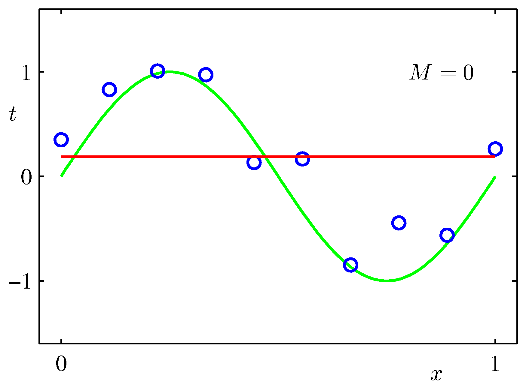
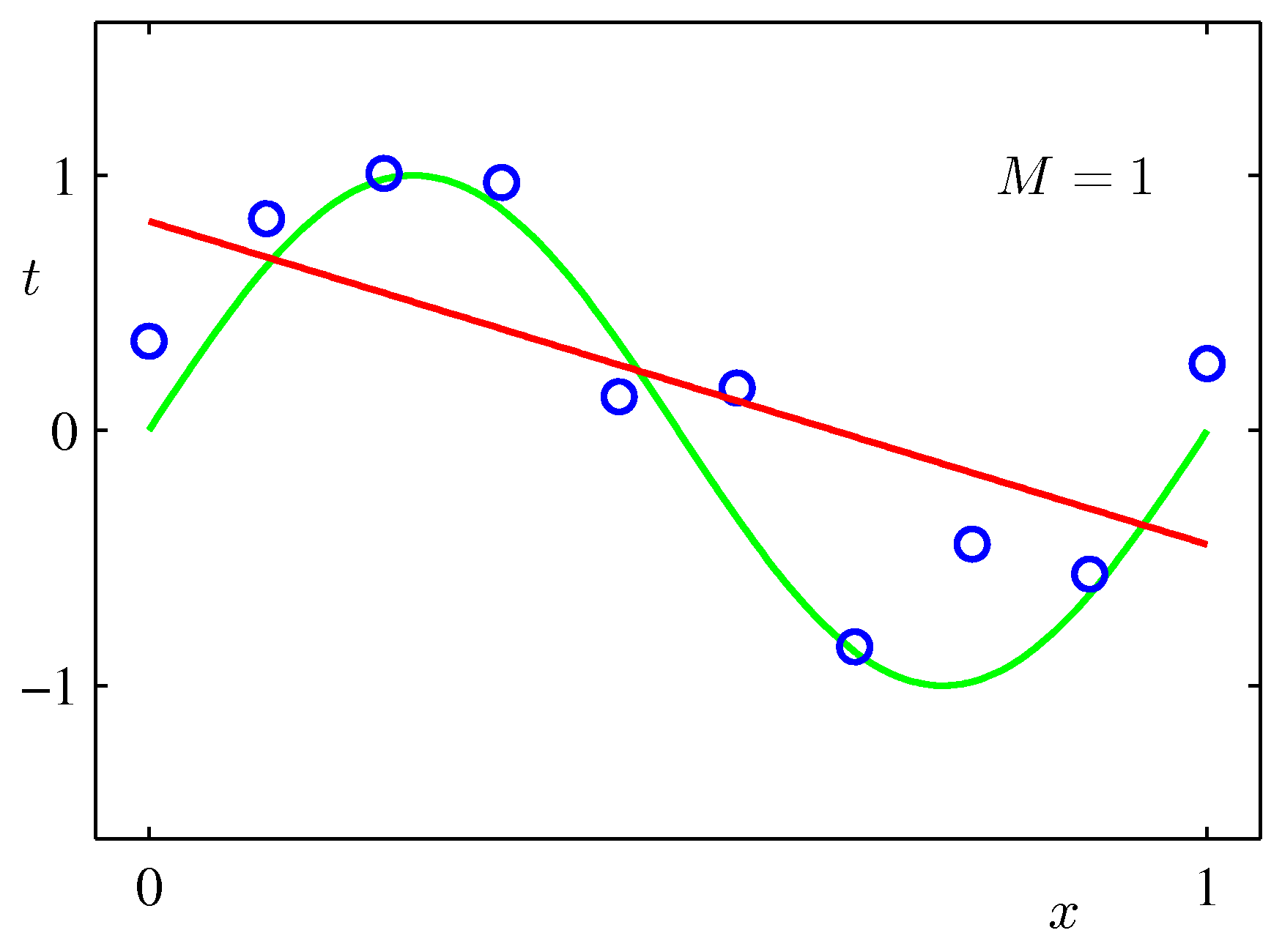
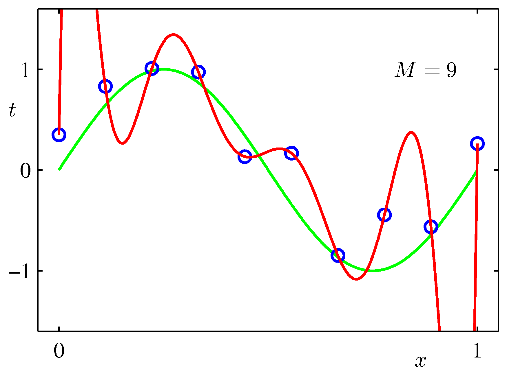
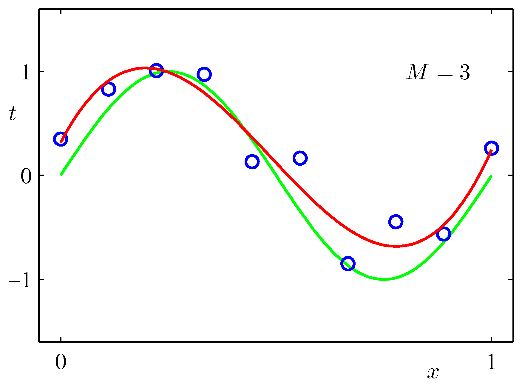
To illustrate the bias-variance tradeoff, we use four examples of the results of fitting polynomials having orders $M=0, 1, 3$ and $9$ to the data.
- $M=0$ (A flat line): $\hat{y} = w_0$
- $M=1$ (A straight slanted line): $\hat{y} = w_0 + w_1x$
- $M=3$ (A smooth cubic curve): $\hat{y} = w_0 + w_1x + w_2x^2 + w_3x^3$
- $M=9$ (A highly flexible curve): $\hat{y} = w_0 + w_1x + w_2x^2 + \cdots + w_9x^9$
5.2 The Three Scenarios (Varying Complexity)
If we fit these different models to our noisy data points, we observe three very distinct behaviors:
Scenario A: $M = 0$ and $M=1$ (High Bias / Underfitting)
- What happens: The models are rigid, straight lines. The polynomials give rather poor fits to the data and consequently rather poor representations of the function $\sin(2\pi x)$. They are mathematically incapable of bending to capture the curve of the data.
- The result: It performs poorly on the training data and poorly on new data.
- The concept: This is known as high bias or underfitting. The model makes strong, incorrect assumptions about the data (assuming a curved relationship is a straight line). We can also say that the model's complexity is too low to capture the variability in the data.
Scenario B: $M = 9$ (High Variance / Overfitting)
- What happens: The model has massive flexibility ($x^9$). It is so eager to minimise the training loss to zero that it bends, twists, and oscillates wildly to pass through every single noisy training point perfectly.
- The result: The training error is exactly zero. However, if you give it a new data point from the true sine wave, the model's prediction will be miles away because it is tracking the noise, not the signal.
- The concept: This is known as high variance or overfitting. The model is highly sensitive to the specific training data sample it saw. If you changed just one data point, the entire $M=9$ curve would swing radically.
Scenario C: $M = 3$ (The Sweet Spot / Generalisation)
- What happens: The cubic polynomial has just enough flexibility to model the underlying smooth curve, but not enough to chase the individual noisy spikes.
- The result: It captures the true underlying physical process. It might not hit every training point perfectly, but it generalises beautifully to unseen test data.
5.3 Understanding the Trade-Off
We can mathematically break down the expected prediction error of any ML model into three distinct components:
- Bias: Error caused by overly simplistic assumptions. (Decreases as model complexity increases).
- Variance: Error caused by over-sensitivity to the specific training data. (Increases as model complexity increases).
- Irreducible Noise ($\epsilon$): The fundamental randomness in the data that no model can ever fix.
The above equation equation is saying: the total prediction error is the sum of error from the model being too simple, error from being too complex (unstable), and error that cannot be eliminated at all. In practice, good modelling is about reducing the first two as much as possible, while accepting that the last one will always remain.
If we observe the behaviour of the training and test set the error for various values of $M$, we see that the test error decreases at first and then shoots very high when $M=9$. The Bias-Variance Trade-off is the quest to find the lowest point on this U-shaped test error curve shown above.
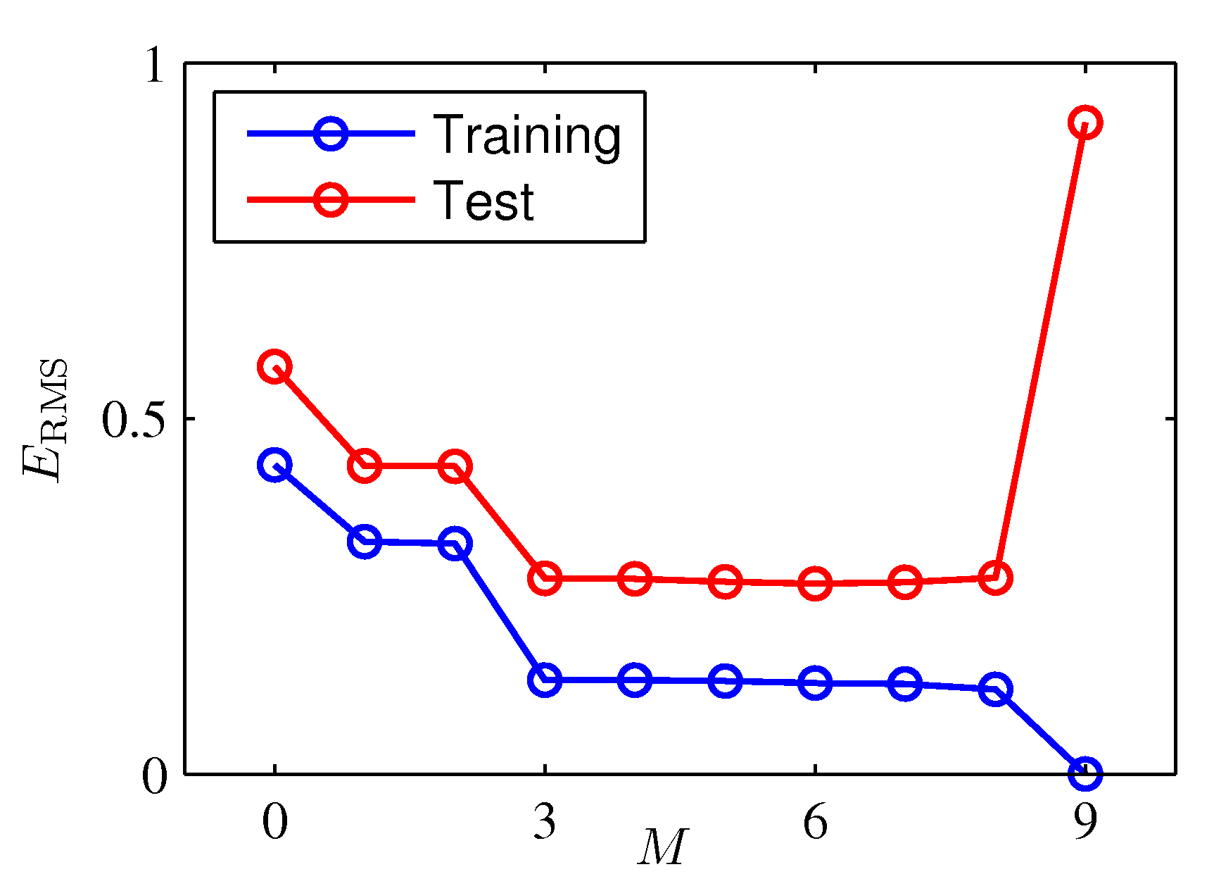
5.4 Diagnosing the Issue Using Error (Loss) Curves
How do you know if your model is suffering from high bias or high variance in production? You plot the training error and validation error together against model complexity (or training epochs).
- If you see: Both Training Error and Validation Error are high → High Bias (Underfitting). Your model hasn't learned the pattern yet.
- If you see: Training Error is very low, but Validation Error is very high (a massive gap between the two curves) → High Variance (Overfitting). Your model has memorised (overfit to) the training set.
5.5 Remedy Toolkit
| If your model has High Bias (Underfitting)... | If your model has High Variance (Overfitting)... |
|---|---|
| 1. Increase complexity: Move from a linear model to a polynomial or a neural network. | 1. Add more training data: More data forces the model to learn the global pattern instead of local noise. |
| 2. Add more features: Give the model more information to work with. | 2. Apply Regularisation: Penalise large weights (e.g., $L_1$/$L_2$ regularization) to keep the curve smooth. |
| 3. Reduce Regularisation: Stop holding the model back; let it learn. | 3. Reduce Complexity: Drop the polynomial degree or use fewer features. |
6. Model Evaluation
Objective: Move beyond simple "accuracy" to evaluate models using metrics that match the high-stakes reality of real-world problems.
When evaluating a model, the most intuitive question to ask is: "What percentage of the time was the model right?" This is accuracy. However, accuracy is highly deceptive when dealing with imbalanced datasets (where one class is much more common than the other).
Imagine you are building a model to detect a rare disease that only affects 1% of the population. If you write a completely useless model that just guesses "Healthy" for every single patient, your model will be 99% accurate. But it is 100% useless because it misses every sick person.
To prevent this, we use a more granular set of tools.
6.1 The Confusion Matrix: The Source of Truth
Every advanced classification metric is derived from a $2 \times 2$ grid called a confusion matrix. It cross-references what the model predicted against what the true answer actually was.
| Pred\Actual | Sick (Class 1) | Healthy (Class 0) |
|---|---|---|
| Sick (Class 1) | True Positive (TP) | False Positive (FP) — Type I Error |
| Healthy (Class 0) | False Negative (FN) — Type II Error | True Negative (TN) |
- True Positive (TP): Sick person correctly predicted as Sick.
- True Negative (TN): Healthy person correctly predicted as Healthy.
- False Positive (FP) [Type I Error]: Healthy person mistakenly predicted as Sick (False Alarm).
- False Negative (FN) [Type II Error]: Sick person mistakenly predicted as Healthy (Missed Case).
6.2 Precision vs. Recall: The Strategic Trade-off
Instead of looking at the whole matrix at once, we often care about specific types of mistakes. This brings us to the two most critical metrics in classification:
A. Precision
- Tells us the quality of the model's positive predictions.
- We ask, "Out of all the points the model predicted as positive, how many were actually positive?"
- When to use: When the cost of a False Positive (False Alarm) is incredibly high.
- Example — Spam Filtering: If a model has low precision, it will flag an important email from your boss as "Spam" (False Positive). We prefer a model that lets a little spam through rather than one that hides critical emails.
B. Recall / Sensitivity
- Tells us what proportion of positive cases were captured by the model.
- We ask, "Out of all the actual positive points in the dataset, how many did the model manage to find?"
- When to use: When the cost of a False Negative (Missed Case) is catastrophic.
- Example — Medical Diagnosis or Cancer Detection: If a patient has cancer and the model misses it (False Negative), they go untreated. We would much rather have a False Alarm (high recall, lower precision) that can be cleared up with a secondary test than miss a life-threatening condition.
C. The F1-Score
- Strikes a balance between precision and recall
- If you want a single metric that balances both without letting a model cheat by favoring one over the other, you use the F1-Score. It is the harmonic mean of Precision and Recall:
6.3 ROC-AUC: Threshold-Independent Evaluation
Classification models don't just output "0" or "1"; they output a probability score (e.g., "This image has an 82% chance of being a cat"). By default, we use a threshold of 0.5 to make the final decision.
If we change that threshold, our Precision and Recall values will shift. To evaluate a model regardless of the threshold chosen, we use the ROC Curve (Receiver Operating Characteristic) and calculate the AUC (Area Under the Curve).
- The curve: Plots the True Positive Rate (Recall) against the False Positive Rate at every possible classification threshold.
- The AUC Score: Ranges from 0 to 1.
- $\text{AUC} = 0.5$: The model is as good as flipping a random coin.
- $\text{AUC} = 1.0$: A perfect model that separates the classes flawlessly.
6.4 Regression Metrics: Measuring Numerical Error
If you are predicting a continuous number (like temperature or biomass) instead of a category, you can't use a confusion matrix. You must use distance-based error metrics. Here are a few commonly used ones:
| Metric | Formula | Practical Meaning |
|---|---|---|
| MAE (Mean Absolute Error) | $\frac{1}{n}\sum \lvert y - \hat{y} \rvert$ | The average size of the mistake. It treats all errors equally. |
| MSE (Mean Squared Error) | $\frac{1}{n}\sum(y - \hat{y})^2$ | Squares the errors before averaging. Penalises large outlier mistakes heavily. |
| RMSE (Root Mean Squared Error) | $\sqrt{\text{MSE}}$ | Puts the MSE back into the original units of the target variable (e.g., dollars or meters), making it easier to interpret. |
Question: Imagine an autonomous vehicle braking system. If it detects an obstacle, it slams on the brakes. Do we design the ML model powering this system to maximise Precision or Recall? Why?
Answer: Recall. A False Positive means the car brakes randomly for a shadow or a plastic bag (annoying but safe). A False Negative means the car fails to brake for an actual pedestrian (catastrophic). We must catch every single true positive obstacle.
7. Parametric vs Non-Parametric Models
Objective: Learn how to categorise machine learning algorithms based on the fundamental assumptions they make about the shape of your data.
When picking an algorithm for a project, one of the most powerful mental shortcuts you can use is deciding whether you need a Parametric or a Non-Parametric model. This distinction tells you instantly how much data you will need, how fast the model will train, and how flexible it will be.
7.1 Parametric Models
A parametric model makes a strong assumption about the underlying shape or functional form of the data before it even looks at a single data point. It assumes the data fits a specific mathematical blueprint.
Because the shape is fixed, the model only needs to learn a specific, constant number of parameters (weights). No matter how massive your dataset grows, the number of parameters remains exactly the same.
Think of a parametric model like a cookie cutter. No matter what kind of dough (data) you throw at it, it will always try to stamp out a specific shape. Some classic examples are:
- Linear Regression (Assumes the relationship is a perfect straight line: $y = wx + b$).
- Logistic Regression (Assumes the data can be separated by a smooth S-curve/sigmoid).
- Linear Discriminant Analysis (LDA).
- Incredibly Fast: They require very little computational power to train and make predictions.
- Data Efficient: They can work well even with relatively small datasets because the "blueprint" guides them.
- Highly Interpretable: It is easy to look at the final mathematical formula and see exactly how each feature affects the prediction.
- High Bias: If your real-world data doesn't fit the blueprint (e.g., you try to fit a straight line to highly complex, twisting data), the model will perform terribly. It is fundamentally limited by its assumptions.
7.2 Non-Parametric Models
A non-parametric model makes zero assumptions about the functional form of the data. It does not look for a straight line or a specific curve. Instead, it allows the structure of the model to grow and adapt dynamically based entirely on the training data it sees. Think of a non-parametric model like play-dough. It molds itself entirely to the shape of the data points around it.
The term "non-parametric" is slightly misleading—it doesn't mean the model has no parameters. It means the number of parameters is not fixed. The parameters grow and change as you add more data points. Here are some examples:
- K-Nearest Neighbors (KNN): Makes predictions purely based on the closest surrounding data points.
- Decision Trees / Random Forests: Splits the data into smaller and smaller rectangular boxes based on feature thresholds.
- Support Vector Machines (SVM) with non-linear kernels.
- Highly Flexible: They can fit highly complex, non-linear patterns that a parametric model could never capture.
- Low Bias: You don't have to worry about making the wrong assumption about your data's shape beforehand.
- Prone to High Variance (Overfitting): Because they are so flexible, they are highly susceptible to memorising the noise in your training set if left unchecked.
- Computationally Heavy: They often require storing and searching through the training data to make predictions (like KNN), making them slower and memory-intensive.
- Data Hungry: They require a lot more data to reliably map out the underlying patterns without getting lost in the noise.
7.3 Summary
| Property | Parametric Models | Non-Parametric Models |
|---|---|---|
| Assumptions | Strong (Assumes a fixed mathematical shape) | None (Learns the shape from data) |
| Number of Parameters | Fixed (Constant) | Flexible (Grows with dataset size) |
| Training Speed | Extremely fast | Slower / Resource intensive |
| Best Used When... | You have smaller data, need speed, or understand the data's true physics. | You have lots of data, complex relationships, and no pre-existing assumptions. |
If you know your data follows a straight line, use a parametric model; it's elegant and lightning-fast. If your data looks like a messy, unpredictable maze, throw a non-parametric model at it; it will carve out a path organically.