Objective: Define the linear regression model rigorously, beginning with simple straight lines and then generalising to flexible combinations of features, and finally express the entire system compactly using matrix notation.
The goal of regression is to predict the value of one or more continuous target variables $t$ given the value of a $D$-dimensional vector $\mathbf{x}$ of input variables. The polynomial fitting example we encountered in the previous lesson is an example of a regression problem. The polynomial is a specific example of a broad class of functions called linear regression models, which share the property of being linear functions of the adjustable parameters.
1. The Linear Regression Model Formulation
Linear regression in its simplest form produces models that are linear in the input variables. A far richer class of functions, however, arises when we form linear combinations of a predetermined set of nonlinear transformations of the inputs—these transformations are called basis functions. Because the model is linear in the parameters, it retains convenient analytical properties (closed-form estimators, straightforward regularisation, etc.), while allowing nonlinear dependence on the inputs through the chosen basis functions.
Given a training dataset comprising $N$ observations $\{\mathbf{x}_n\}$, where $n=1, \cdots, N$, together with corresponding target values $\{t_n\}$, the goal is to predict the value of $t$ for a new value of $\mathbf{x}$. In the simplest approach, this can be done by directly constructing an appropriate function $y(\mathbf{x})$ whose values for new inputs $\mathbf{x}$ constitute the predictions for the corresponding values of $\mathbf{t}$.
1.1 The Core Model: Linear in the Parameters
In basic statistics, a linear relationship between a single input $x$ and a target $y$ is written as $\hat{y} = w_0 + w_1x$. In machine learning, we need to extend this to handle multiple input features and highly non-linear patterns. We can do this by passing our raw inputs through the basis functions before applying our weights.
The general linear regression model is defined as:
- $\mathbf{w} = (w_0, w_1, \dots, w_{M-1})^T$ is the vector of model parameters (weights).
- $w_0$ is the bias parameter (or intercept), which allows the model to shift vertically away from the origin.
- $\phi_j(x)$ is a basis function. It takes the raw input $x$ and transforms it.
- $M$ is the total number of parameters in the model.
Why is this still called linear regression if the basis functions can be non-linear? Because the model is strictly linear in the parameters $\mathbf{w}$. The parameters only multiply the features linearly; they are never squared, passed into a sine wave, or raised to a power. This property ensures the optimisation landscape remains convex (a bowl shape), making it easy to solve.
1.2 Common Choices for Basis Functions
By choosing different basis functions ($\phi$), we can change the types of patterns our model can fit:
- Linear Basis (Identity): $\phi_j(x) = x_j$. This is standard multiple linear regression, where the inputs are used exactly as they are.
- Polynomial Basis: $\phi_j(x) = x^j$. This allows us to fit curves (like the $M=3$ sine wave approximation we discussed previously).
- Gaussian Basis: Takes a localized approach, mapping data based on its distance from a specific center $\mu_j$:
To make the math elegant, we don't want to treat the bias $w_0$ as a special exception outside the summation. We introduce a "dummy" basis function, $\phi_0(x) = 1$. This allows us to write the entire summation compactly as a vector dot product:
where $\mathbf{w} = [w_0, w_1, \dots, w_{M-1}]^T$ and $\boldsymbol{\phi}(x) = [\phi_0(x), \phi_1(x), \dots, \phi_{M-1}(x)]^T$.
1.3 Scaling Up: The Design Matrix ($\Phi$)
When we have a real dataset, we don't just have one input $x$; we have a collection of $N$ data points (observations). We need a clean way to compute all predictions simultaneously without using slow loop structures.
Suppose our dataset contains $N$ input samples: $\{\mathbf{x}_1, \mathbf{x}_2, \dots, \mathbf{x}_N\}$. If we pass every single sample through our $M$ basis functions, we stack them vertically to create the Design Matrix, denoted by the capital Greek letter $\Phi$ (Phi).
- Shape of $\Phi$: It is an $N \times M$ matrix ($N$ rows of samples, $M$ columns of transformed features).
- Because $\phi_0(\mathbf{x}) = 1$, the very first column of the Design Matrix is always a column of $1$s.
Using this Design Matrix, we can express the predictions for our entire dataset as a single matrix-vector multiplication:
where $\mathbf{\hat{y}}$ is an $N \times 1$ vector containing the predicted target values for every single instance in the dataset.
- $\Phi$ has shape $N \times M$
- $\mathbf{w}$ has shape $M \times 1$
- Therefore, $\Phi \mathbf{w}$ yields an $(N \times 1)$ output vector, matching the exact shape of our true target labels $\mathbf{y}$.
2. The Objective: Maximum Likelihood & Ordinary Least Squares (OLS)
Objective: Ground the choice of the sum-of-squares error function in probability theory using Maximum Likelihood Estimation (MLE), and explore its geometric interpretation.
2.1 The Probabilistic Framework (Maximum Likelihood)
When solving the polynomial fitting problem in the previous lesson, we minimised a sum of squares error function:
Before going any further with these formulae, let's understand how a data point is born in the real world. Imagine you are measuring tree heights based on their age. There is an underlying, perfect physical law of nature (our model, $\mathbf{w}^T \boldsymbol{\phi}(x)$). If nature were perfect, a 5-year-old tree would always be exactly 10 meters tall.
But the real world has noise ($\epsilon$)—wind shaking your measuring laser, genetic variation, or soil differences. So, your actual measurement ($y$) is:
What is "Inverse Variance"?
Variance ($\sigma^2$), is a measure of how "spread out" a distribution is. If a sensor is cheap and shaky, it has high variance. If it is a high-grade laboratory instrument, it has low variance. For now, we will introduce the new term Precision ($\beta$), not to be confused with the metric used with classification, which is simply the inverse of variance:
- High Precision (Large $\beta$): The noise is tiny. Your measurements are tightly clustered around the true line.
- Low Precision (Small $\beta$): The noise is huge. Your data points are wildly scattered far away from the line.
Using $\beta$ just makes our algebra cleaner later on because it keeps the variable in the numerator rather than the denominator.
The Gaussian Distribution of a Guess?
Because the noise $\epsilon$ is random and symmetric, we assume it follows a standard Gaussian (bell curve) centered at zero. If we shift that bell curve so that it is centered right on top of our model's clean prediction, we get the probability of seeing a specific target $y$:
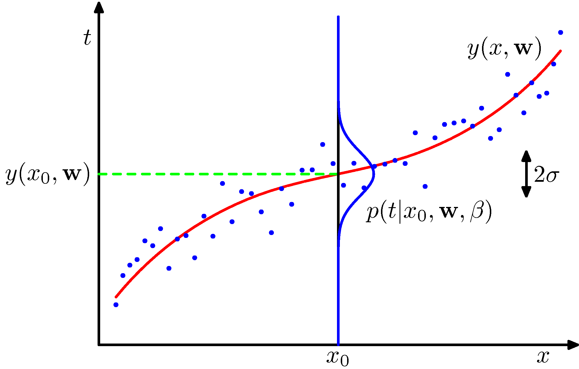
Look at the diagram above. The line is where the model thinks the data should be. The bell curves show the probability of where the data point actually lands. A point close to the line has high probability; a point far up or down in the tails of the curve has very low probability.
Intuition of "Maximum Likelihood"
Now, what does Maximum Likelihood Estimation (MLE) actually mean? Imagine I show you a scatter plot of data points, and I draw two different lines through it:
- Line A: Passes directly through the middle of the dense cluster of points.
- Line B: Is drawn far away in the empty top corner of the graph.
If I ask you, "Which line is more likely to be the true relationship?" you would instantly pick Line A. Why? Because the data points are close to it. Under Line A's bell curves, your data points have high probability scores. Under Line B, your data points sit out in the extreme tails where the probability is practically zero.
Maximum Likelihood is simply the mathematical way of saying: "Find the line that makes the data we actually observed look as normal and expected as possible."
2.2 Connecting the Probability to the Core Math
If we have $N$ independent data points, the total "likelihood" of our entire dataset is found by multiplying the individual probabilities of every single point together:
More compactly written as:
Because multiplying fractions yields tinier fractions (which computers hate of something called numerical instability), we take the Logarithm. The log turns multiplication into addition:
More compactly:
Using the laws of logarithms ($\ln(ab) = \ln a + \ln b$), we can pull this apart:
We want to find the parameter vector $\mathbf{w}$ that maximizes this log-likelihood. Look closely at the final equation: the first two terms do not depend on $\mathbf{w}$ at all. The only term containing $\mathbf{w}$ has a negative sign in front of it (i.e., the summation term). The other terms can be ignored because they do not depend on $\mathbf{w}$.
To make the Total Likelihood as large as possible, we need to make this negative subtraction term as small as possible. Therefore, maximizing the log-likelihood with respect to $\mathbf{w}$ is mathematically equivalent to minimizing the summation term. And what is $(y_i - \mathbf{w}^T \boldsymbol{\phi}(x_i))^2$? It is the squared distance between the actual data point and our line. Therefore, we define this summation as our Sum-of-Squares Error Function, $E_D(\mathbf{w})$:
We ignore $\beta$ because it does not change the location of the global minimum that we seek.
So, we have just completed the formal proof that Ordinary Least Squares (OLS) is the optimal solution under the assumption of normally distributed noise.
2.3 Geometric Interpretation of Least Squares
Imagine an $N$-dimensional space where each axis represents a single data point in our training set.
- The true target labels vector $\mathbf{y} = (y_1, \dots, y_N)^T$ forms a single vector in this $N$-dimensional space.
- Each column of our Design Matrix $\Phi$ can also be viewed as a vector in this same space. There are $M$ such columns, and together they span an $M$-dimensional linear subspace (often called the data manifold or column space).
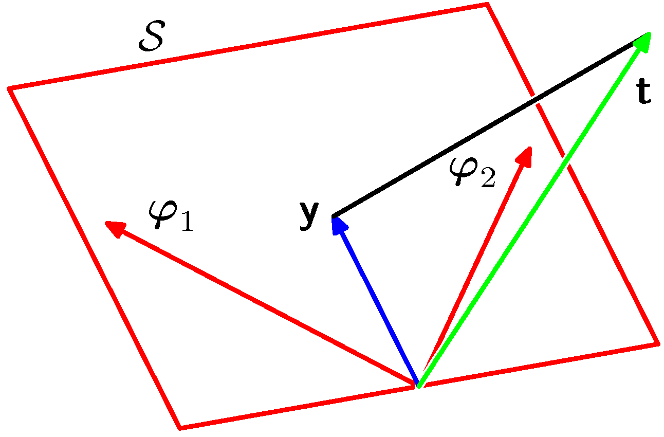
Because $\mathbf{\hat{y}} = \Phi \mathbf{w}$, any prediction our model can possibly make must lie somewhere within this $M$-dimensional subspace. Our goal is to find a prediction vector $\mathbf{\hat{y}}$ that is as close as possible to the true target vector $\mathbf{y}$. Geometrically, the shortest distance from a point ($\mathbf{y}$) to a plane (our subspace) is a straight, perpendicular line.
Therefore, the least-squares solution for $\mathbf{w}$ corresponds to the orthogonal projection of the target vector $\mathbf{y}$ onto the subspace spanned by the columns of $\Phi$.
2.4 Summary
- Probabilistic perspective: Minimizing squared errors means maximizing the probability of observing our dataset if the noise is Gaussian.
- Geometric perspective: Minimizing squared errors means dropping a perpendicular line from our true answers onto the mathematical space spanned by our input features.
We shall now proceed to understand how to solve the linear programming problem by finding the OLS solution.
3. Approach 1: The Analytical Solution (Linear Algebra)
Objective: Derive the exact, closed-form solution for the optimal weight vector $\mathbf{w}$ using matrix calculus, and understand its computational limits.
3.1 Minimizing the Error Function
From our previous section, our objective is to minimize the sum-of-squares error function:
Using the design matrix $\Phi$ and the target vector $\mathbf{y}$ introduced in Section 1, we can rewrite this entire summation compactly in matrix notation as:
To find the vector $\mathbf{w}$ that minimizes this error, we use vector calculus. We need to take the gradient of $E_D(\mathbf{w})$ with respect to $\mathbf{w}$ and set it equal to zero.
3.2 Computing the Gradient
Let's expand the matrix error function first to make the differentiation clear:
Now, we compute the gradient vector $\nabla_{\mathbf{w}} E_D(\mathbf{w})$ by applying standard rules of matrix (or multivariate) calculus:
- $\frac{\partial}{\partial \mathbf{w}} (\mathbf{w}^T \mathbf{A} \mathbf{w}) = 2\mathbf{A}\mathbf{w}$ (for a symmetric matrix $\mathbf{A}$)
- $\frac{\partial}{\partial \mathbf{w}} (\mathbf{w}^T \mathbf{b}) = \mathbf{b}$
Applying these rules yields:
3.3 The Normal Equation
To find the global minimum, we set this gradient vector to a vector of zeros ($\mathbf{0}$):
Rearranging the terms gives us the famous Normal Equation:
To solve for $\mathbf{w}$, we multiply both sides from the left by the inverse of the matrix $(\Phi^T \Phi)$, assuming it is invertible:
This represents the exact, analytical solution to the Ordinary Least Squares problem.
3.4 The Moore-Penrose Pseudo-Inverse
The quantity $(\Phi^T \Phi)^{-1} \Phi^T$ is known as the Moore-Penrose pseudo-inverse of the design matrix $\Phi$, denoted as $\Phi^\dagger$ (read as "Phi dagger").
The pseudo-inverse generalizes the concept of a matrix inverse to non-square matrices (refer to Section 3.1.1 in Bishop's book for a deeper discussion on its properties).
3.5 ⚠️ When does this approach fail?
The analytical solution requires that the $M \times M$ matrix $(\Phi^T \Phi)$ is strictly invertible. It will fail or become highly unstable in two real-world scenarios:
- Multicollinearity: When two or more features are perfectly correlated (e.g., measuring weight in both pounds and kilograms). This creates redundant columns in $\Phi$, making the matrix singular (non-invertible).
- Data Scarcity ($N < M$): If you have more features/parameters ($M$) than data points ($N$), the matrix $(\Phi^T \Phi)$ will not have full rank, meaning it has an infinite number of perfect solutions, leading to extreme overfitting.
Inverting an $M \times M$ matrix has a computational complexity of approximately $O(M^3)$. If your model uses 100,000 features, computing $(\Phi^T \Phi)^{-1}$ requires roughly $10^{15}$ operations! This heavy computational cost is exactly why we need iterative approaches like Gradient Descent.
4. Approach 2: The Iterative Solution (Gradient Descent)
Objective: Understand how to find the optimal weights using an iterative optimization process, providing an efficient alternative when computing the analytical solution is too costly.
4.1 Why Switch to an Iterative Approach?
In the previous section, we found a perfect, exact formula for the optimal weights: $\mathbf{w} = (\Phi^T \Phi)^{-1} \Phi^T \mathbf{y}$.
However, computing the term $(\Phi^T \Phi)^{-1}$ requires inverting an $M \times M$ matrix, which takes $O(M^3)$ computational time. If you are dealing with millions of features or large-scale deep learning models, doing a matrix inversion is computationally impossible.
Instead of jumping directly to the answer in a single step, we can use Gradient Descent to start with random weights and gradually alter them to find the minimum of our error function.
4.2 The Batch Gradient Descent Update Rule
Recall that the gradient of our sum-of-squares error function (from Section 3) is:
To find the minimum, we want to step in the direction opposite to the gradient (downward into the valley). The iterative update rule is written as:
Where:
- $t$ represents the current iteration step.
- $\eta$ (Eta) is the learning rate (a hyperparameter controlling step size).
If we substitute our explicit gradient into this formula, we get the Batch Gradient Descent update rule:
Look at the term $(\mathbf{w}^T \boldsymbol{\phi}(x_i) - y_i)$. This is simply the prediction error for data point $i$. The algorithm calculates the error, multiplies it by the feature values ($\boldsymbol{\phi}(x_i)$), and sums this up across all $N$ data points to make a single update to the weight vector.
4.3 Sequential Learning: Stochastic Gradient Descent (SGD)
The Batch Gradient Descent rule has one major drawback: it requires looking at every single one of your $N$ data points just to make a single, tiny adjustment to $\mathbf{w}$. If $N$ is in the millions, this is incredibly slow.
To overcome this, we can update our weights sequentially, processing one data point at a time. This is known as Stochastic Gradient Descent (SGD), or the Least-Mean-Squares (LMS) algorithm (refer to Section 3.1.3 in Bishop's book).
For a single observed data point $i$, the update rule becomes:
4.4 Comparing the Behaviors
- Batch Gradient Descent: Follows a smooth, direct path straight down to the minimum because it calculates the true gradient using the entire dataset. However, each step is computationally expensive.
- Stochastic Gradient Descent: Takes fast, cheap steps, but its path to the minimum is highly erratic and zig-zagged because individual data points can be noisy or outliers.
4.5 Summary Matrix: Analytical vs. Iterative
| Property | Analytical (Normal Equation) | Iterative (Gradient Descent) |
|---|---|---|
| Mathematical Goal | Solve $\nabla E_D(\mathbf{w}) = \mathbf{0}$ directly. | Tweak $\mathbf{w}$ until $\nabla E_D(\mathbf{w}) \approx \mathbf{0}$. |
| Computational Cost | $O(M^3)$ — Scale limits are bound by number of features. | $O(M \cdot N)$ per iteration (or $O(M)$ for SGD). |
| Hyperparameters | None. | Must carefully tune the learning rate $\eta$. |
| Best Used When... | Dataset is small enough to fit in memory ($M < 10{,}000$). | Dataset or feature space is massive ($M$ or $N$ is very large). |
Linear regression represents a rare luxury in machine learning because its error landscape is perfectly convex, meaning it has a single global minimum. Whether you slide down analytically or walk down iteratively, you are guaranteed to reach the exact same optimal destination.