1. Introduction and Conceptual Overview
In this section, we will explore the transition from linear models—such as linear regression and linear classification—to adaptive, non-linear neural networks. The goal is to understand why multi-layer perceptrons (MLPs) are designed the way they are, tracing their origins from their early biological inspiration to today's mathematically rigorous computational architectures.
1.1 From Linear Models to Non-linear Representations
1.1.1 The Limitations of Linear Models
In previous discussions, we examined linear models for regression and classification. A typical linear regression model takes an input vector $\mathbf{x} = [x_1, x_2, \dots, x_D]^T$ and predicts a target value using a linear combination of the inputs:
Where:
- $\mathbf{w} = [w_1, w_2, \dots, w_D]^T$ is the weight vector determining the importance and direction of each feature's contribution.
- $b$ is the bias parameter, shifting the decision boundary or regression line away from the origin.
While linear models are computationally attractive because their loss surfaces are convex (making optimisation straightforward), they possess a fundamental limitation: they can only form linear decision boundaries or linear prediction surfaces. If the true underlying relationship between the inputs and targets is non-linear, a pure linear model will suffer from high bias (underfitting).
1.1.2 Fixed Basis Functions and the Curse of Dimensionality
To extend linear models to handle non-linear data without losing their nice optimisation properties, we discussed how to transform the input space using a set of fixed, non-linear functions called basis functions, denoted by $\phi_j(\mathbf{x})$.
The model then becomes:
By collecting the basis functions into a vector $\boldsymbol{\phi}(\mathbf{x}) = [\phi_1(\mathbf{x}), \phi_2(\mathbf{x}), \dots, \phi_{M-1}(\mathbf{x})]^T$, this can be compactly written as:
While this looks like a non-linear model with respect to the input $\mathbf{x}$, it remains linear with respect to the parameters $\mathbf{w}$. This means standard linear algebra techniques can still be used to find the optimal weights. Common choices for fixed basis functions include:
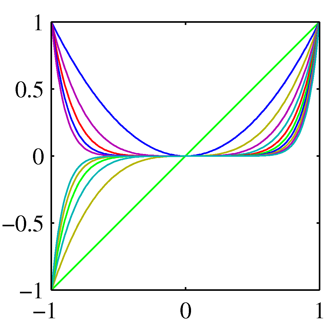
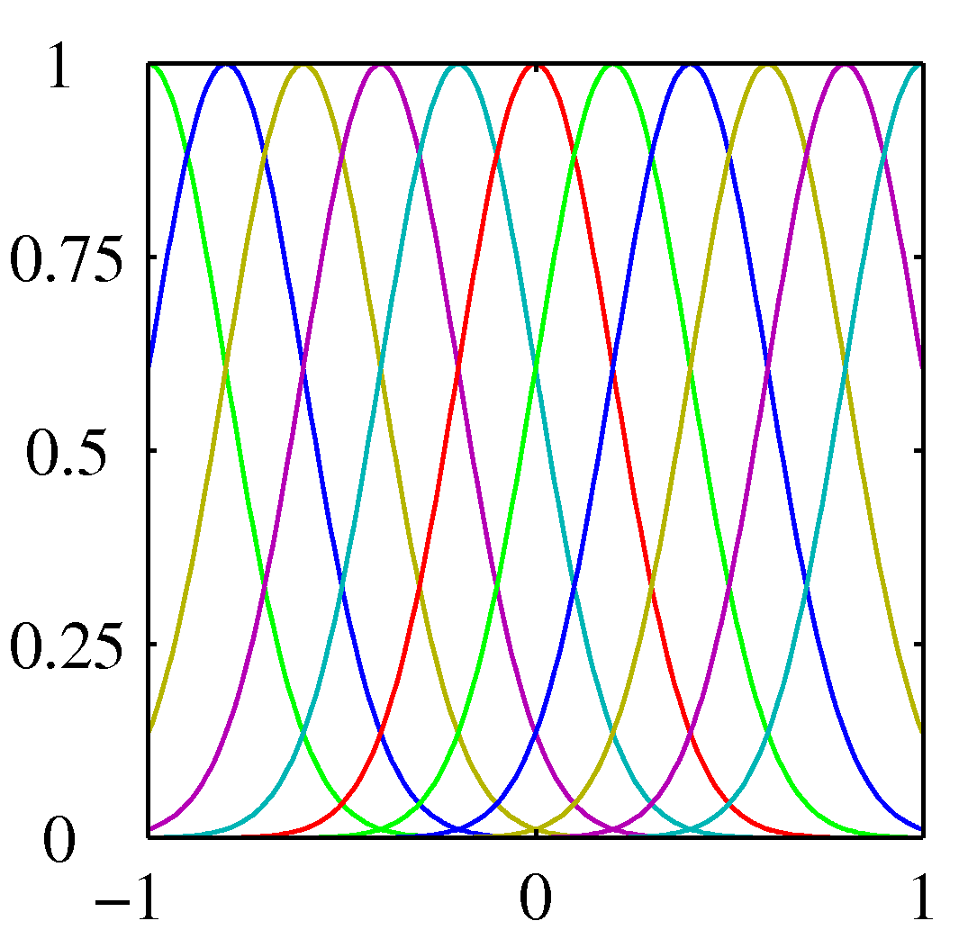
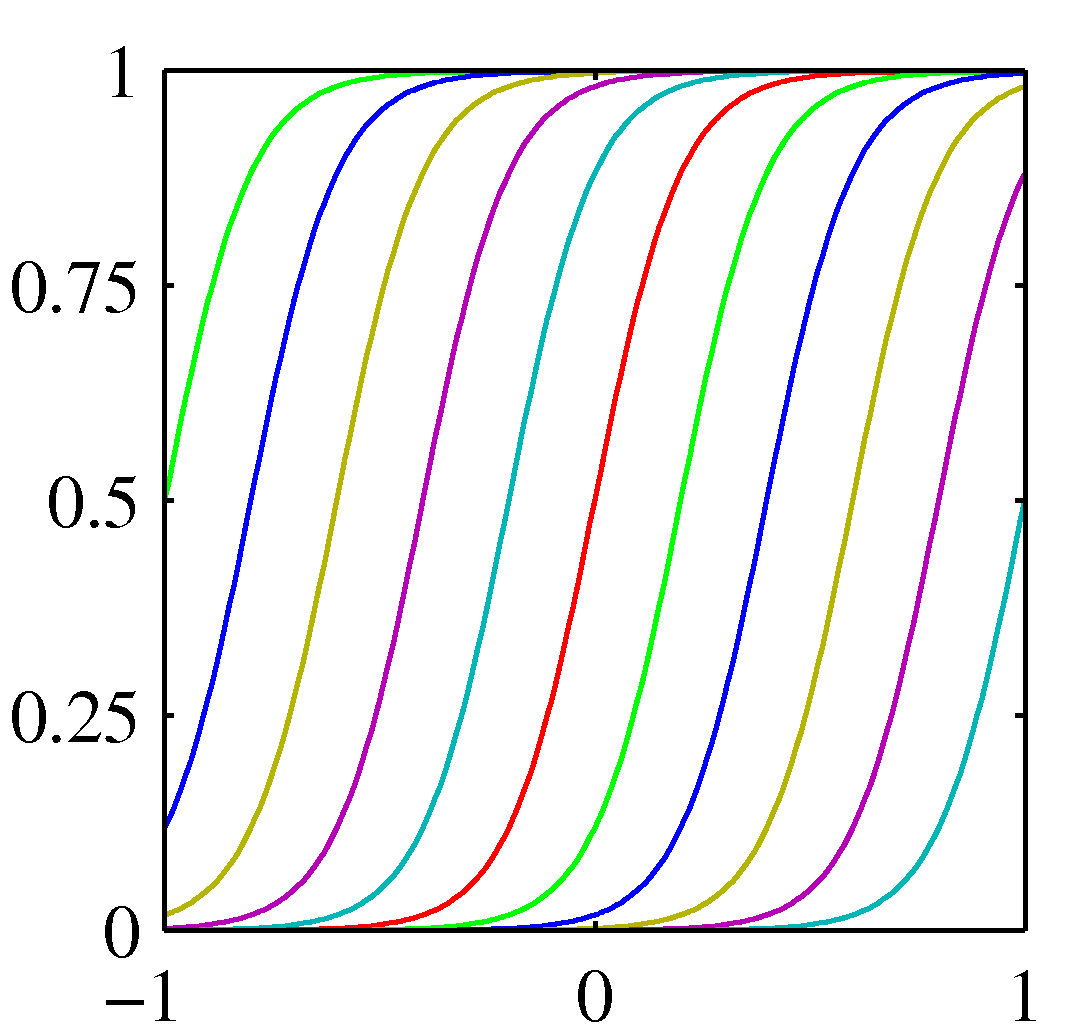
- Polynomial basis functions: $\phi_j(x) = x^j$
- Gaussian basis functions: $\phi_j(x) = \exp \left( -\frac{(x - \mu_j)^2}{2s^2} \right)$
- Sigmoidal basis functions: $\phi_j(x) = \sigma \left( \frac{x - \mu_j}{s} \right)$
The Breakdown of Fixed Basis Functions
Why not simply use this approach for all machine learning problems? The issue lies in the curse of dimensionality.
If the input space $\mathbf{x}$ has a high dimensionality $D$, and a polynomial or grid-based combination of basis functions is chosen to capture fine details, the number of required basis functions $M$ grows exponentially with $D$. For instance, if 10 basis functions are placed along each dimension for a 3-dimensional input space, $10^3 = 1{,}000$ basis functions are needed. For a 100-dimensional input space (such as a small $10 \times 10$ pixel image), $10^{100}$ basis functions would be required—a number that vastly exceeds the number of atoms in the observable universe.
Therefore, manually designing or pre-allocating fixed basis functions becomes completely intractable for high-dimensional data.
1.1.3 Fixed vs. Adaptive Basis Functions
Neural networks resolve this limitation by making the basis functions adaptive. Instead of choosing $\phi_j(\mathbf{x})$ beforehand and keeping it fixed, the parameters that define the basis functions themselves are learned simultaneously with the output weights.
In a neural network, each basis function $\phi_j(\mathbf{x})$ is parameterised by its own set of internal weights and biases:
Where $\sigma(\cdot)$ is a non-linear activation function. The complete model now becomes a multi-layered function where the data determines the most optimal features to extract. This bypasses the curse of dimensionality because the model only constructs the specific basis functions necessary to solve the given task, rather than tiling the entire input space uniformly.
1.2 The Biological vs. Computational Metaphor
1.2.1 Historical Context: The Birth of Artificial Neurons
The conceptual origins of neural networks began with an attempt to model the biological processing mechanisms of the human brain.
In 1943, Warren McCulloch and Walter Pitts introduced the McCulloch-Pitts Neuron, a highly simplified mathematical abstraction of a biological brain cell. In biology, a neuron receives electrochemical signals through its dendrites. If the sum of these signals exceeds a specific threshold, the neuron fires an electrical impulse down its axon to other neurons.
The McCulloch-Pitts model mimicked this by taking binary inputs $x_i \in \{0, 1\}$, summing them, and checking if the sum exceeded a threshold $\theta$:
This early model lacked a mechanism for learning; the thresholds and connections had to be designed by hand.
1.2.2 Rosenblatt's Perceptron
In 1958, Frank Rosenblatt extended this concept by introducing adjustable weights, creating the Perceptron. The Perceptron forms a linear combination of real-valued inputs, adds a bias, and passes the result through a step activation function:
Where the activation function $f(a)$ is a rigid step function:
Rosenblatt developed an iterative learning algorithm to automatically adjust the weights $\mathbf{w}$ based on classification errors. If a training example was misclassified, the weights were adjusted in the direction of the error.
1.2.3 The Linear Barrier: Minsky & Papert's Critique
In 1969, Marvin Minsky and Seymour Papert published a rigorous mathematical critique of the Perceptron. They proved that because a single perceptron is fundamentally a linear classifier, it is entirely incapable of solving problems where the classes are not linearly separable.
The classic example they used was the Exclusive OR (XOR) logical function, where the outputs are defined as:
- $\text{XOR}(0, 0) = 0$
- $\text{XOR}(1, 1) = 0$
- $\text{XOR}(1, 0) = 1$
- $\text{XOR}(0, 1) = 1$
Because no straight line can separate the zeroes from the ones in a 2D plane for the XOR problem, a single Perceptron fails. Minsky and Papert correctly noted that adding a hidden layer of neurons could solve this issue, but they argued that there was no known computationally efficient way to train the weights of those hidden layers. This critique led to a significant reduction in neural network research funding for over a decade, a period often referred to as the first "Artificial Intelligence Winter."
1.2.4 The Transition to Continuous Activation Functions
The breakthrough that revitalised the field was the realisation that neural networks could be trained using calculus-based optimisation (gradient descent) if the rigid, discontinuous step functions of the perceptron were replaced with continuous, differentiable activation functions.
A step function has a derivative of zero everywhere except at the boundary, where it is undefined. A derivative of zero provides no information about which direction to move the weights to reduce the error. By using smooth functions like the logistic sigmoid function:
The function becomes fully differentiable, meaning $\frac{\partial y}{\partial \mathbf{w}}$ can be computed. This non-zero gradient serves as a directional guide, allowing the network to use the chain rule of calculus to calculate how changes to early weights in the network affect the final output error. This foundation forms the basis of the backpropagation algorithm.
1.3 Architectural Paradigms
1.3.1 Definition of a Feedforward Neural Network / Multi-Layer Perceptron (MLP)
The Multi-Layer Perceptron (MLP), also known as a Feedforward Neural Network, consists of multiple layers of computational units ordered such that information flows strictly in one direction: from the input layer, through one or more hidden layers, to the output layer.
The term "feedforward" distinguishes these networks from Recurrent Neural Networks (RNNs). In a feedforward network, there are no feedback loops; the output of any given layer cannot loop back to influence itself or any preceding layer.
1.3.2 Directed Acyclic Graphs (DAGs)
Mathematically, a feedforward network can be formalised as a Directed Acyclic Graph (DAG).
- Graph: A collection of nodes (neurons) connected by edges (weights).
- Directed: Each edge has a specific direction, indicating that node $i$ passes its output value to node $j$.
- Acyclic: There are no paths or closed loops that allow an information signal to travel from a node and eventually return to that same node.
Representing the network as a DAG allows the mathematical computation to be broken down into an ordered sequence of operations, which is crucial for implementation in modern automatic differentiation libraries.
1.3.3 Layer Taxonomy
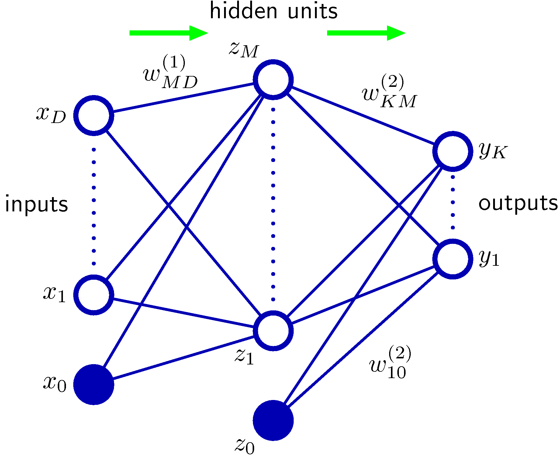
An MLP is typically structured into three distinct types of layers:
Inputs (x) ---> [ Hidden Layer 1 ] ---> [ Hidden Layer 2 ] ---> Outputs (y)
- Input Layer: This layer does not perform any mathematical operations or transformations. It simply represents the raw feature vector $\mathbf{x} = [x_1, x_2, \dots, x_D]^T$ extracted from the environment (e.g., pixel intensities, physical measurements, or sensor readings).
- Hidden Layers: These layers are called "hidden" because their intermediate values are not directly observed in the training dataset; the dataset only provides the inputs and the final target outputs. Each hidden layer extracts increasingly abstract features from the representations provided by the previous layer.
- Output Layer: This final layer transforms the representations generated by the last hidden layer into the network's final prediction $\hat{\mathbf{y}}$. The structure and mathematical activation of this layer are entirely determined by the specific machine learning task being performed (e.g., continuous values for regression or probabilities for classification).
Next, we develop the precise mathematical matrix equations that govern how information travels forward through this network layout, alongside an analysis of different activation functions.
2. The Feedforward Architecture
In this section, the precise mathematical mechanisms that govern how information flows through a Multi-Layer Perceptron (MLP) will be formalised. We have already noted that neural networks bypass the curse of dimensionality by constructing adaptive basis functions. We will now construct the exact algebraic equations of these adaptive units, demonstrate how they compose into hierarchical layers, and explore how their final outputs are tailored to match specific probabilistic targets.
2.1 The Single-Neuron Functional Unit
The fundamental building block of a feedforward neural network is the individual processing node, often called a hidden unit or an artificial neuron. This unit performs two successive mathematical transformations on its inputs: a linear combination followed by a non-linear activation.
2.1.1 The Linear Combination
Let a single neuron receive an input vector $\mathbf{x} = [x_1, x_2, \dots, x_D]^T$ from the preceding layer. The unit first computes a weighted sum of these inputs and adds a scalar bias parameter $b$. This combined scalar value is called the pre-activation, denoted by $a$:
Where $\mathbf{w} = [w_1, w_2, \dots, w_D]^T$ is the parameter vector assigned to this specific neuron. The weight vector determines the orientation of the neuron's decision plane, while the bias $b$ shifts the activation threshold away from the origin.
2.1.2 The Activation Function
To convert the pre-activation $a$ into a useful adaptive feature, it is passed through a non-linear activation function $\sigma(\cdot)$ to produce the post-activation value $z$:
As already discussed, this activation function must be continuous and differentiable to permit gradient-based learning. The choice of $\sigma(\cdot)$ fundamentally alters the optimisation landscape and the types of functions the network can easily represent.
2.1.3 Properties and Trade-offs of Common Activation Functions
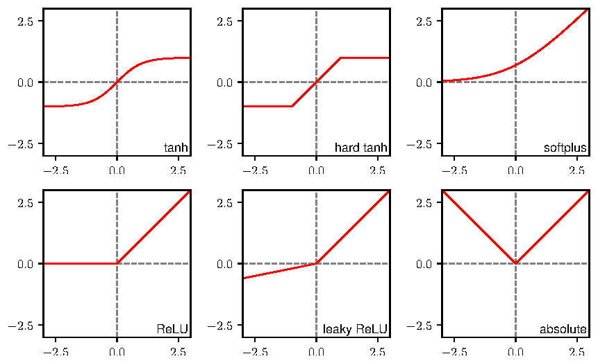
1. The Sigmoid (Logistic) Function
The sigmoid function squashes any real-valued input into a strictly bounded range between 0 and 1:
- Mathematical Property: Its derivative can be expressed compactly in terms of its output: $\sigma'(a) = \sigma(a)(1 - \sigma(a))$
- Limitation (Saturation): When the pre-activation $a$ becomes very large or very small (large negative), the curve flattens out, causing the gradient $\sigma'(a)$ to approach zero. This leads to the vanishing gradient problem, where weight updates down the line stall completely during backpropagation.
2. The Hyperbolic Tangent ($\tanh$)
The $\tanh$ function is a closely related, scaled version of the sigmoid function, mapping inputs into a range between -1 and 1:
- Advantage: Unlike the sigmoid, the $\tanh$ function is zero-centered (its output has an expected value close to zero when inputs are symmetrically distributed). This makes optimisation more stable because the gradients in subsequent layers do not all shift systematically in the same positive or negative direction.
- Limitation: It still suffers from saturation at extreme values of $a$.
3. The Rectified Linear Unit (ReLU)
In modern neural network architectures, the ReLU activation has largely replaced sigmoidal functions in hidden layers. It is defined as a simple piecewise linear function:
- Advantage: For any positive pre-activation ($a > 0$), the derivative is exactly 1 ($f'(a) = 1$). This completely eliminates the vanishing gradient problem for positive activations, allowing deep architectures to train significantly faster. It is also exceptionally cheap to compute.
- Limitation (Dying ReLU): For any negative pre-activation ($a < 0$), both the output and the derivative are exactly zero. If a neuron gets updated such that it always receives negative inputs across the entire dataset, its gradient remains zero forever, and it becomes a "dead neuron" that can no longer learn.
4. Leaky ReLU and GeLU
To mitigate the dying ReLU problem, variants with small non-zero gradients for negative inputs are utilised:
- Leaky ReLU: Introduces a small constant slope $\alpha$ (typically $0.01$)
when $a < 0$:
$$f(a) = \max(\alpha a, a)$$
- Gaussian Error Linear Unit (GeLU): Used extensively in state-of-the-art
transformer and deep MLP networks. It weights the input by its probability under a
standard normal cumulative distribution function:
$$f(a) = a \cdot \Phi(a)$$This creates a smooth, deterministic approximation of the ReLU that preserves a slight curvature for negative values.
2.2 Multi-Layer Composition (Matrix Formulation)
When individual neurons are aggregated into a layer, and several layers are stacked sequentially, computing the network's forward pass by iterating through individual nodes becomes notationally and computationally inefficient. Instead, compact linear algebra expressions are used.
2.2.1 Forward Propagation Equations for a Single Hidden Layer
Consider a network with an input layer, one hidden layer containing $M$ hidden units, and an output layer containing $K$ units.
Let the input vector be $\mathbf{x} \in \mathbb{R}^D$.
- The weight parameters for the entire hidden layer can be collected into a matrix $\mathbf{W}^{(1)}$ of size $M \times D$, where each row $j$ represents the weight vector $\mathbf{w}_j^{(1)}$ for hidden unit $j$.
- The bias parameters are collected into a vector $\mathbf{b}^{(1)} \in \mathbb{R}^M$.
The vector of pre-activations $\mathbf{a}^{(1)} \in \mathbb{R}^M$ for the hidden layer is computed simultaneously as:
Applying the element-wise non-linear activation function $\sigma(\cdot)$ yields the hidden layer's output vector (or post-activation vector) $\mathbf{z} \in \mathbb{R}^M$:
The vector $\mathbf{z}$ now acts as the newly transformed, adaptive basis representation of the input $\mathbf{x}$ (directly connecting back to the concept in Section 1.1). This hidden representation is passed to the output layer, which has its own weight matrix $\mathbf{W}^{(2)}$ of size $K \times M$ and bias vector $\mathbf{b}^{(2)} \in \mathbb{R}^K$. The output pre-activations $\mathbf{a}^{(2)} \in \mathbb{R}^K$ are computed as:
Finally, the network's raw predictions $\hat{\mathbf{y}} \in \mathbb{R}^K$ are obtained by passing these values through an output activation function $f(\cdot)$:
2.2.2 Generalisation to $L$ Layers
This mathematical formulation scales naturally to an arbitrary depth $L$. For any intermediate hidden layer $l \in \{1, 2, \dots, L\}$, the sequence of operations can be written recursively as:
Where $\mathbf{z}^{(0)} = \mathbf{x}$ represents the baseline input features, and $\hat{\mathbf{y}} = \mathbf{z}^{(L)}$ represents the final network output. Written out completely, an MLP is a nested functional composition:
This demonstrates that despite the complexity of the functions a deep neural network can learn, the entire inference process consists entirely of alternating matrix multiplications and element-wise non-linear mappings.
2.3 Network Output Layer Design & Probabilistic Interpretation
The choice of the final layer activation function $f\left(\mathbf{a}^{(L)}\right)$ is not arbitrary. It is dictated entirely by the statistical nature of the target variables in the training set. By matching the output activation to a specific conditional probability distribution, the network's predictions can be interpreted rigorously within a Maximum Likelihood Estimation framework.
2.3.1 Linear Outputs for Continuous Regression
When the task is to predict a vector of continuous, unconstrained target values $\mathbf{t} \in \mathbb{R}^K$, a linear output activation is used:
From a probabilistic perspective, this assumes that the true target $\mathbf{t}$ is equal to the deterministic network prediction $\hat{\mathbf{y}}$ corrupted by additive, zero-mean Gaussian noise:
Where $\beta^{-1}$ is the variance of the noise. Maximising the likelihood under this assumption directly yields the Mean Squared Error (MSE) objective.
2.3.2 Sigmoid Outputs for Binary Classification
If the task is a binary classification problem where the target belongs to one of two classes, $t \in \{0, 1\}$, the network must output a single scalar value representing the conditional probability $p(t=1 \mid \mathbf{x})$. Because a probability must be strictly bounded between 0 and 1, the logistic sigmoid activation function is applied to the final pre-activation:
This models the conditional class distribution as a Bernoulli distribution:
2.3.3 Softmax Outputs for Multi-class Classification
When a mutually exclusive classification problem involves $K > 2$ distinct classes, the target is represented as a one-hot encoded vector $\mathbf{t} \in \{0, 1\}^K$ where exactly one element equals 1. The network requires $K$ output units, and their values must form a valid probability distribution (each output must be greater than zero, and the sum of all $K$ outputs must equal 1).
To achieve this, the softmax function is applied to the output pre-activation vector $\mathbf{a}^{(L)}$:
- Interpretation: The softmax function takes a vector of unconstrained real values (often called "logits") and exponentiates them to ensure they are strictly positive, then normalises them by dividing by the sum of all exponentiated values.
- Probabilistic Model: This maps directly to a Multinomial (or Categorical)
distribution over the classes:
$$p(\mathbf{t} \mid \mathbf{x}, \mathbf{w}) = \prod_{k=1}^K \hat{y}_k^{t_k}$$
The above equation is a fancy way of saying "Given the input $\mathbf{x}$ and model parameters $\mathbf{w}$, the probability that the target/class vector is $\mathbf{t}$ is exactly the predicted probability of the chosen class, and zero for the others, written in a compact product form."
For example, suppose the correct class $j$. Then $t_j=1$ and $t_k=0$ for all $k\neq j$ (For standard ML problems, the target class can always be thought of as a one-hot vector because for each input vector $\mathbf{x}$, there is typically only one correct class). The product becomes:
Which is just like saying: "The probability of the observed class is the model's predicted probability for that label."
2.4 Expressive Power & Representation
Now that the complete forward pass has been defined, it is vital to discuss the boundaries of what this architecture can theoretically compute.
2.4.1 The Universal Approximation Theorem
One of the foundational theoretical justifications for using neural networks is the Universal Approximation Theorem (proven by George Cybenko in 1989 for sigmoidal functions, and later generalised by Kurt Hornik in 1991).
The theorem states that:
A feedforward neural network with a single hidden layer, containing a finite number of neurons, can approximate any continuous function on a compact subset of $\mathbb{R}^D$ to any desired degree of accuracy, provided the activation function is continuous, bounded, and non-linear.
This is a powerful statement. It guarantees that even a shallow network with just one hidden layer can theoretically represent any smooth mapping we encounter in machine learning.
2.4.2 The Curse of Dimensionality for MLPs
If a single hidden layer is theoretically sufficient, why does modern machine learning focus almost exclusively on deep networks with dozens or hundreds of layers?
The Universal Approximation Theorem is an existence proof; it proves that such a network exists, but it does not tell us how many hidden units are required, nor does it guarantee that standard learning algorithms (like gradient descent) can successfully find the optimal weight parameters.
- Exponential Efficiency of Depth: To approximate complex, highly oscillating functions, a shallow network often requires an exponentially large number of hidden units ($M \to \infty$). This brings back the curse of dimensionality from an architectural standpoint.
- Hierarchical Feature Extraction: Deep networks bypass this limitation by substituting sheer horizontal width with vertical depth. Each layer constructs a new level of abstraction. The first layer might extract simple localised edges, the second layer composes these edges into shapes, and subsequent layers compose shapes into complex semantic objects. This compositional hierarchy allows deep networks to represent intricate functions using a fraction of the total parameters required by a shallow, wide counterpart.
In the next module, the framework for assessing the accuracy of these network outputs will be constructed by deriving formal loss functions, alongside an analysis of the high-dimensional geometric landscapes across which parameters must be optimised.
3. Parameter Optimisation and Loss Surfaces
With the forward pass equations established, the network can now transform an input $\mathbf{x}$ into a prediction $\hat{\mathbf{y}}$. However, at initialisation, the weights $\mathbf{W}$ and biases $\mathbf{b}$ are random, meaning the predictions will be highly inaccurate. We now focus on how to quantify these inaccuracies using loss functions derived from probability theory, explore the geometric landscape of parameters, and examine the optimisation algorithms used to update them.
3.1 Error Functions via Maximum Likelihood Estimation (MLE)
In introductory machine learning contexts, error functions (or loss functions) are sometimes introduced as heuristic measures of distance. We already saw that we can derive loss functions systematically using the principle of Maximum Likelihood Estimation (MLE).
Let a dataset consist of $N$ independent and identically distributed (i.e., i.i.d.) observations $\mathbf{X} = \{\mathbf{x}_1, \dots, \mathbf{x}_N\}$ with corresponding target labels $\mathbf{T} = \{\mathbf{t}_1, \dots, \mathbf{t}_N\}$. Depending on the task, we will apply one of the following error functions for optimisation:
3.1.1 Mean Squared Error (MSE) for Regression
For a continuous regression problem where we predict a target vector $\mathbf{t}_n$ assumed to be corrupted by additive Gaussian noise with precision (inverse variance) $\beta$, we saw that minimising $E(\mathbf{w})$ with respect to the network weights $\mathbf{w}$ reduces to minimising:
If we set the scaling multiplier $\frac{\beta}{2}$ to an arbitrary constant (commonly $\frac{1}{2}$ or $\frac{1}{N}$), the standard Mean Squared Error (MSE) function is obtained:
3.1.2 Binary Cross-Entropy (BCE) for Binary Classification
For binary classification, where $t_n \in \{0, 1\}$ and the output $\hat{y}_n = \sigma(a_n)$, we use the binary cross-entropy loss function:
3.1.3 Categorical Cross-Entropy for Multi-class Classification
For multi-class classification with $K$ mutually exclusive classes, the target $\mathbf{t}_n$ is a one-hot vector and the output $\hat{\mathbf{y}}_n$ is generated via the softmax activation function. The categorical cross-entropy loss function is:
3.2 Geometry of the Error Surface
Once an error function $E(\mathbf{w})$ is selected, it can be viewed geometrically as a surface suspended over the high-dimensional parameter space. If a network has $W$ parameters, the error surface exists in a $(W+1)$-dimensional space.
3.2.1 The Loss Surface Landscape
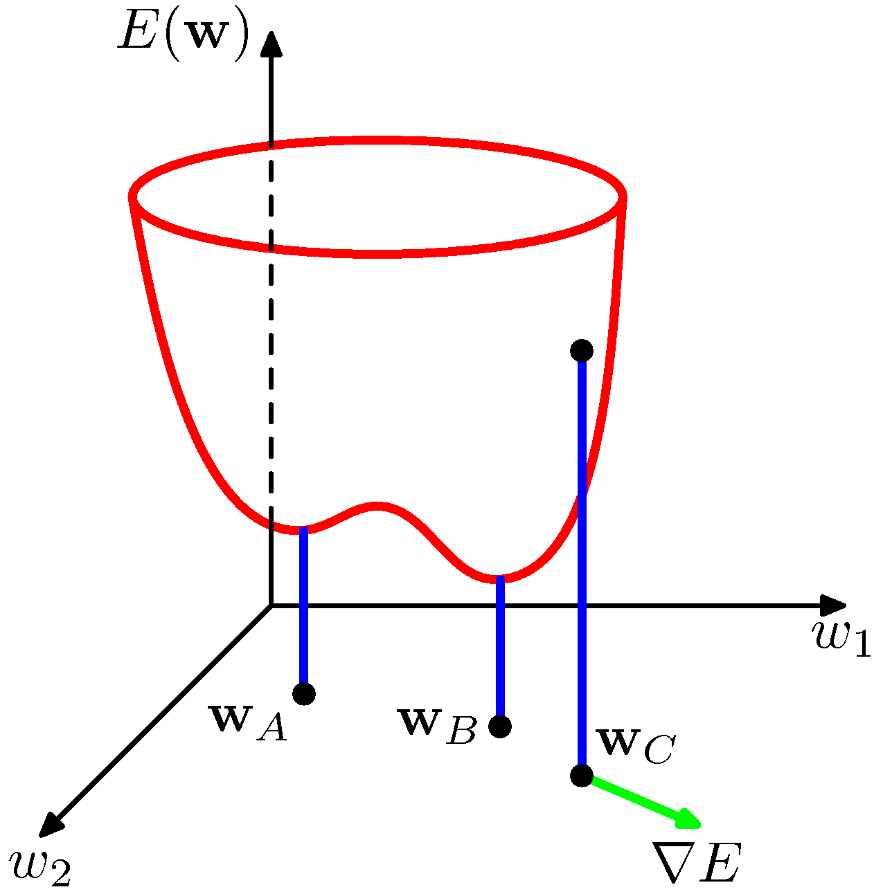
In linear regression, the error surface is a perfectly convex paraboloid, containing a single global minimum that is easy to locate. However, because neural networks compose non-linear activation functions hierarchically, the resulting loss surface $E(\mathbf{w})$ is highly non-convex. It contains distinct geometric features:
- Global Minima: Parameter configurations that yield the absolute lowest possible error value.
- Local Minima: Regions where the error is lower than in the immediate surrounding neighborhood, but higher than the global minimum.
- Saddle Points: Points where the surface slopes upward along some parameter dimensions but downward along others.
The tools required to analyse the local geometry of this surface mathematically to determine whether we arrived at a local or global minimum or saddle point are beyond our scope. In summary, certain properties of the Hessian matrix $H$ of the error function's $E(\mathbf{w})$ determine what optima the optimisation process yields:
- If all eigenvalues of $H$ are strictly positive, the region is a local minimum.
- If all eigenvalues of $H$ are strictly negative, the region is a local maximum.
- If there is a mix of positive and negative eigenvalues in $H$, the region is a saddle point.
3.2.2 High-Dimensionality in Modern Neural Networks
Early neural network literature focused heavily on the risk of getting trapped in poor local minima. However, in modern deep networks where $W$ can span millions or billions of dimensions, the geometric reality is different.
For a point to be a true local minimum, the slope must curve upward in every single one of the $W$ dimensions simultaneously—meaning all eigenvalues of $\mathbf{H}$ must be positive. The probability of this occurring randomly in high dimensions is exceptionally low. Instead, the vast majority of critical points ($\nabla E = 0$) encountered in large networks are saddle points. Optimisation algorithms must therefore be capable of traversing these flat saddle regions efficiently without stalling.
3.3 Gradient Descent Variants
To find a parameter configuration that minimises $E(\mathbf{w})$, the network relies on iterative optimisation algorithms. The foundational algorithm is Gradient Descent, which uses the gradient vector $\nabla E(\mathbf{w})$ to determine the direction of steepest descent.
3.3.1 Batch Gradient Descent (BGD)
In Batch Gradient Descent, the exact gradient of the total error function is computed by evaluating every single training sample in the dataset before performing a parameter update:
Where $\eta > 0$ is the learning rate (or step size) and $\tau$ denotes the iteration index.
- Limitation: If the dataset contains millions of samples, computing $\nabla E$ requires tracking every sample through the network just to make a single update step. This is computationally slow and requires more memory than a standard system possesses.
3.3.2 Stochastic Gradient Descent (SGD)
Stochastic Gradient Descent addresses this limitation by updating the parameter weights immediately after processing a single, randomly selected training example $\mathbf{x}_n$:
- Advantage: Parameter updates are computed quickly, and new data can be processed on the fly.
- Limitation: Because a single sample provides a noisy approximation of the true gradient across the entire dataset, the optimisation path fluctuates significantly. While this variance can help the parameters escape shallow saddle points, it prevents the algorithm from settling cleanly into a minimum, causing it to oscillate continuously around it.
3.3.3 Mini-batch Stochastic Gradient Descent
The standard approach in modern machine learning is Mini-batch SGD, which strikes a practical balance between the stability of batch gradient descent and the speed of stochastic gradient descent. The dataset is partitioned into small subsets $\mathcal{B}$ called mini-batches, typically containing $B$ samples (e.g., $B = 32, 64, \text{ or } 256$).
The update formula is defined as:
| Optimisation Variant | Gradient Variance | Computational Efficiency | Hardware Utilisation |
|---|---|---|---|
| Batch ($B=N$) | Zero variance (Exact) | Very low per step | Poor (Does not leverage parallel processing at scale) |
| Stochastic ($B=1$) | High variance (Noisy) | High per step | Extremely poor (Cannot utilise matrix operations) |
| Mini-batch ($1 < B < N$) | Controlled variance | High and balanced | Excellent (optimised for matrix vectorisation on hardware) |
Mini-batch SGD reduces the noise in the gradient updates compared to pure SGD, while leveraging highly optimised matrix algebra libraries on computing hardware to process multiple samples in parallel.
In the next module, the algorithmic core of neural network training will be explored: the backpropagation algorithm, analysing how the local error signals ($\delta$) and structural partial derivatives are passed backward through the layers of our computational graph.
4. The Backpropagation Algorithm
In the previous section, it was established that to improve a network's performance, parameters must be updated by moving in the opposite direction of the gradient:
The gradient vector $\nabla E$ is simply a collection of partial derivatives. For any single weight $w_{ji}$ in the network, the exact value of $\frac{\partial E}{\partial w_{ji}}$ must be calculated to know how a tiny change in that specific weight impacts the total error $E$.
The Backpropagation algorithm is the standard method used to compute these derivatives efficiently. While it is often viewed as complex, backpropagation relies entirely on a single rule from introductory calculus: the Chain Rule. In this section, we break down the algorithm into straightforward steps using basic algebra.
4.1 Mathematical Foundations: The Chain Rule
4.1.1 The Single-Variable Chain Rule
Consider a situation where a variable $y$ depends on $u$, and $u$ depends on $x$. If a small change is made to $x$, it alters $u$, which in turn alters $y$. To find out how fast $y$ changes with respect to $x$, the rates of change are multiplied together:
4.1.2 The Multi-Variable Chain Rule
In a neural network, a single hidden unit can pass its output to multiple units in the next layer. This requires the multi-variable version of the chain rule. If a variable $x$ influences a final variable $E$ through multiple independent paths (for example, through intermediate variables $a_1$ and $a_2$), the total effect is the sum of the changes along each individual path:
4.2 Derivation of the Backward Pass
Let's look at a single connection inside a network. Suppose a weight $w_{ji}$ connects the output of node $i$ (which we call $z_i$) to the input of node $j$ in the next layer.
The mathematical operations occur in a specific sequence:
- Compute the pre-activation: Node $j$ sums all its weighted inputs to calculate $a_j = \sum_{i} w_{ji} z_i + b_j$.
- Apply the activation function: This value is passed through a non-linear function to get $z_j = \sigma(a_j)$.
- Forward flow: This output continues through the remaining layers until it reaches the final error $E$.
To evaluate how the weight $w_{ji}$ affects the error $E$, the single-variable chain rule is applied:
This expression consists of two distinct parts that can be solved individually.
4.2.1 Part 1: Evaluating $\frac{\partial a_j}{\partial w_{ji}}$
The term $a_j$ is defined by the equation $a_j = w_{j1}z_1 + w_{j2}z_2 + \dots + w_{ji}z_i + \dots + b_j$. If we take the derivative of $a_j$ with respect to the specific weight $w_{ji}$, all other terms drop out because they do not depend on $w_{ji}$:
This demonstrates that the first part of the derivative is simply the incoming signal ($z_i$) passing through that weight.
4.2.2 Part 2: The Local Error Signal ($\delta_j$)
The remaining part of our chain rule equation measures how a change in the pre-activation $a_j$ affects the total error. This is defined as the local error signal or the delta value of node $j$:
Substituting both components back into the main chain rule equation yields a straightforward final formula:
The derivative of the error with respect to any weight is simply the local error ($\delta_j$) at the receiving node multiplied by the input signal ($z_i$) from the sending node.
Similarly, for the bias parameter $b_j$, because $\frac{\partial a_j}{\partial b_j} = 1$, its derivative simplifies to:
4.3 Computing the Deltas ($\delta$) Backward
To apply this formula across the network, the value of $\delta_j$ must be calculated for every node. This process moves backward, starting from the final layer.
4.3.1 Step 1: Deltas at the Output Layer ($L$)
For a node $k$ in the final output layer, its pre-activation $a_k$ directly influences the output $\hat{y}_k$, which goes straight into the error function $E$. Applying the chain rule reveals:
Using a standard regression problem with a Mean Squared Error loss ($E = \frac{1}{2}(\hat{y}_k - t_k)^2$) and a linear output layer ($\hat{y}_k = a_k$) as an example:
- The derivative of the error is $\frac{\partial E}{\partial \hat{y}_k} = (\hat{y}_k - t_k)$.
- The derivative of the activation function is $\frac{\partial \hat{y}_k}{\partial a_k} = 1$.
Multiplying these together gives the final output delta:
The local error at the final output layer is simply the difference between the network's prediction and the true target value.
4.3.2 Step 2: Deltas at the Hidden Layers (The Recurrence Relation)
For a node $j$ located in a hidden layer, it does not connect directly to the final error. Instead, its pre-activation $a_j$ influences the error by sending its signal to every single node in the next layer ($l+1$).
We need to keep our notation clear and simple. Let indices $i$, $j$, and $k$ represent individual tracking labels for neurons sitting in three consecutive layers of the network:
- $i$ (The sending node in the earlier layer): Represents a neuron in layer $l-1$. It outputs the signal $z_i$, which travels forward across the weight $w_{ji}$.
- $j$ (The current node under evaluation): Represents a neuron in the middle layer $l$. This is the specific node where we are currently trying to calculate the local error signal $\delta_j$ and update its incoming weights $w_{ji}$.
- $k$ (The receiving node in the next layer): Represents a neuron in layer $l+1$. Because a single neuron $j$ sends its output $z_j$ forward to multiple downstream neurons, we use $k$ to loop through and sum up all the different receiving neurons that neuron $j$ impacted.
That is:
- $w_{ji}$: The weight connecting sending node $i$ to receiving node $j$.
- $w_{kj}$: The weight connecting sending node $j$ to receiving node $k$.
To compute $\delta_j$, the multi-variable chain rule is applied to sum up the error signals flowing back from all the receiving nodes $k$ in the next layer:
where:
Using the definitions established above:
- $\frac{\partial E}{\partial a_k}$ is the local error at the next layer, which is $\delta_k$.
- To find $\frac{\partial a_k}{\partial a_j}$, the relationship is broken down into
two parts: $a_k$ depends on $z_j$ (via the weight $w_{kj}$), and $z_j$ depends on
$a_j$ (via the activation function $\sigma$).
$$\frac{\partial a_k}{\partial a_j} = \frac{\partial a_k}{\partial z_j} \cdot \frac{\partial z_j}{\partial a_j} = w_{kj} \cdot \sigma'(a_j)$$
Plugging these back into the summation formula yields the standard backpropagation recurrence equation:
To find the local error ($\delta_j$) at a hidden neuron, take all the errors from the next layer ($\delta_k$), multiply them by the weights connecting them ($w_{kj}$), sum them up, and scale the result by the slope of the current node's activation function ($\sigma'(a_j)$).
4.4 The Step-by-Step Practical Algorithm
To train a network in practice, these mathematical steps are executed in a systematic cycle:
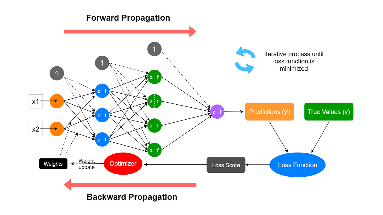
- The Forward Pass: Input a training example $\mathbf{x}$. Compute the activations layer-by-layer moving forward ($\mathbf{a}^{(1)} \to \mathbf{z}^{(1)} \to \mathbf{a}^{(2)} \to \dots$). Keep a record of all intermediate values $a$ and $z$ in memory.
- Output Error Evaluation: Compute the initial error signals $\delta_k$ at the final layer using the prediction error $(\hat{y}_k - t_k)$.
- The Backward Pass: Use the recurrence equation $\delta_j = \sigma'(a_j) \sum w_{kj} \delta_k$ to pass the error signals backward through the hidden layers, calculating a $\delta$ value for every neuron.
- Gradient Calculation: For each individual parameter, multiply the local delta by the incoming activation ($\frac{\partial E}{\partial w_{ji}} = \delta_j z_i$) to find the gradient. Use these gradients to update the weights via gradient descent.
4.5 Computational Efficiency
Evaluating the forward pass requires a specific number of basic operations proportional to the number of weights, $O(W)$. Backpropagation allows the gradients for every single weight to be calculated during the backward pass in roughly the same amount of time, $O(W)$. This efficiency makes training deep networks computationally viable.
Next, our focus shifts to evaluating how well this optimisation process generalises to unseen data, exploring the balance between bias and variance alongside explicit regularisation techniques.
5. Regularisation and Generalisation
In the previous section, we learnt how to use the backpropagation algorithm to calculate gradients and minimise our training error. However, minimising error on our training data is not our ultimate goal. In machine learning, we want our network to perform well on unseen data, that is generalisation.
When a network performs exceptionally well on the training data but fails to predict accurately on new, unseen test data, it has overfit the data. This module explores why this happens and introduces basic mathematical and algorithmic tools to prevent it.
5.1 The Bias-Variance Trade-off and Capacity
To understand generalisation, we must look at the trade-off between two types of errors that affect our model: Bias and Variance.
5.1.1 Bias (Underfitting)
Bias measures how much our model's predictions differ from the true values because the model's architecture is too simple.
- Example: If we try to fit a highly curved dataset using a straight line, the line will never capture the curve, no matter how much training data we give it.
- This is called underfitting. The model has high bias.
5.1.2 Variance (Overfitting)
Variance measures how much our model's predictions change if we train it on a completely different set of data from the same problem.
- Example: If we have a model with millions of parameters (high capacity) and a small dataset, the model can literally memorise the specific noise, quirks, and random fluctuations of those exact training samples.
- When we give it new data, its performance plummets because it tuned itself too specifically to the training set. This is called overfitting. The model has high variance.
5.1.3 The Overfitting in Neural Networks
Because Multi-Layer Perceptrons (MLPs) have high expressive power, they are highly prone to overfitting. If left unchecked, a deep network will bend its decision boundaries excessively to ensure every single training data point is classified perfectly, resulting in poor generalisation. Regularisation is the collective term for techniques used to control a model's capacity and prevent overfitting.
5.2 Explicit Regularisation Techniques
Explicit regularisation works by modifying our original error function $E(\mathbf{w})$ to penalise the network for becoming too complex.
5.2.1 $L_2$ Regularisation (Weight Decay)
The most common form of explicit regularisation adds a penalty term based on the squared magnitude of the weights to the error function. We define our regularised error function $\tilde{E}(\mathbf{w})$ as:
Where:
- $E(\mathbf{w})$ is our standard error function (like MSE or Cross-Entropy).
- $\|\mathbf{w}\|^2 = \sum_{i} w_i^2$ is the sum of all squared weights in the network (biases are typically excluded).
- $\lambda > 0$ is a hyperparameter called the regularisation coefficient that determines how heavily we penalise large weights.
Why does this help? (The Intuition)
To see how this affects our updates, let's look at the gradient of our new error function with respect to a single weight $w$:
When we plug this into our standard Gradient Descent update rule, we get:
Rearranging the terms highlights a clear pattern:
Because $(1 - \eta \lambda)$ is a number slightly less than 1, every single training step automatically shrinks the weight toward zero before adding the standard gradient update. This is why $L_2$ regularisation is widely known as weight decay. Keeping the weights small prevents any single neuron from exerting an overly dominant, highly sensitive influence on the output, creating a smoother, less complex model function.
5.2.2 $L_1$ Regularisation
Alternatively, we can penalise the absolute values of the weights rather than their squares:
The derivative of $|w|$ with respect to $w$ is simply $+1$ if $w$ is positive, and $-1$ if $w$ is negative (written as $\text{sign}(w)$). The update rule becomes:
The Difference: While $L_2$ regularisation shrinks large weights quickly but slows down when weights are near zero, $L_1$ regularisation subtracts a constant force $\eta\lambda$ from the weight regardless of its size. This drives less important weights completely to exactly zero, creating a sparse model where many connections are entirely turned off.
5.3 Architectural & Algorithmic Regularisation
Instead of altering the math of the error function, we can use structural modifications to keep the network from overfitting.
5.3.1 Early Stopping
When training a neural network, we typically monitor both the error on our training set and the error on a separate validation set (data not used for gradient descent updates).
As training progresses over time (epochs):
- The training error steadily decreases as the network learns the data.
- Initially, the validation error decreases alongside it as the network picks up general patterns.
- Eventually, the network begins to overfit, causing the training error to keep dropping while the validation error begins to rise.
Early Stopping is the simple practice of saving the network's parameters at the exact point where the validation error is at its lowest, and stopping the training process before the validation error begins climbing.
5.3.2 Dropout
Dropout is a highly effective regularisation technique developed specifically for deep neural networks. During training, at each forward pass, dropout randomly forces a subset of hidden units to output zero. Each neuron has a probability $p$ (often $0.5$) of being temporarily deactivated for that specific step.
Why does Dropout work?
- Breaks Co-adaptation: In a standard network, neurons can develop unhealthy dependencies on one another, where neuron B relies on neuron A to correct its mistakes. By randomly removing neurons, every hidden unit is forced to learn robust features that are useful independent of the surrounding nodes.
- Approximate Ensembling: Dropping nodes randomly means that for every training step, we are effectively training a slightly different, smaller sub-network. When training completes, we turn all neurons back on but scale their weights down by the probability $(1-p)$ to match the expected signal strength. This means running inference through a fully trained dropout network is mathematically similar to averaging the predictions of thousands of unique networks simultaneously, which significantly boosts generalisation.
5.3.3 Data Augmentation
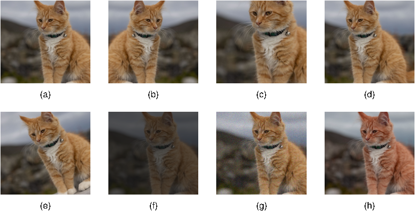
If a network overfits because its capacity is too high for a small dataset, a practical solution is to increase the size of the dataset. If collecting more real-world data is impossible, we can create synthetic variations of our existing data through Data Augmentation.
For image data, this involves applying minor transformations that do not change the core identity of the object:
- Randomly flipping the image horizontally.
- Small rotations or slight cropping modifications.
- Subtle adjustments to brightness or contrast.
By injecting these variations, we explicitly force the network's adaptive basis functions to learn invariants (e.g., a car is still a car whether it faces left, faces right, or is slightly shadowed), making it much more robust when deployed on genuine, unseen test data.
Next, we will explore advanced optimisation techniques—such as momentum and adaptive optimisers like Adam—which help navigate these regularised surfaces efficiently.
6. Advanced Optimisation and Practical Training Considerations
We have already explored how a neural network learns by using gradient descent to find the lowest points on a complex loss surface. In practice, however, standard gradient descent can be slow, inefficient, and prone to stalling. We now cover the conceptual tools and practical techniques used to help networks train faster, bypass geometric obstacles, and start the learning process on the right foot—all without diving into the heavy calculus.
6.1 Momentum and Adaptive Optimisers
When a network relies on basic mini-batch gradient descent, it often struggles to navigate the loss surface. Modern training uses smarter optimisation strategies to accelerate learning.
6.1.1 Momentum: The Rolling Ball Metaphor
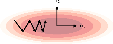
Imagine the optimisation process as a heavy ball rolling down a hilly terrain toward a valley. Standard gradient descent only looks at the slope exactly where the ball is standing right now. If it hits a steep, narrow ravine, it will bounce back and forth violently between the side walls, making very slow progress down the actual length of the valley.
Momentum solves this by introducing physical simulation. It allows the optimisation step to remember its previous velocity.
- As the ball rolls down a consistent slope, it gathers speed, taking larger and larger steps in the correct direction.
- When it encounters erratic, back-and-forth oscillations, the opposing forces cancel each other out, damping the bouncing behavior and keeping the path stable.
- This momentum also helps the optimiser push straight through flat areas (saddle points) where standard gradient descent would lose energy and stall.
6.1.2 RMSprop and Adam: Adaptive Learning Rates
In standard gradient descent, we set a single learning rate for the entire network. However, some weights might have massive gradients (steep cliffs) while others have tiny gradients (flat plains). A single learning rate might be too large for the steep sections (causing crashes) and too small for the flat sections (causing stagnation).
Adaptive optimisers fix this by giving every single weight its own personalized learning rate.
- RMSprop: This method tracks a running average of how volatile each weight's gradient has been. If a weight is experiencing massive, erratic updates, RMSprop automatically scales down its individual learning rate to stabilise it. If a weight has tiny, sluggish updates, it scales up its learning rate to accelerate it.
- Adam (Adaptive Moment Estimation): Think of Adam as the ultimate combination of Momentum and RMSprop. It simultaneously remembers the past direction of travel (Momentum) while dynamically scaling the step size for each individual parameter based on recent volatility (RMSprop). Because of this balance, Adam is the default, go-to optimiser for most modern deep learning projects.
6.2 The Problem of Scale: Initialization and Normalization
Even with advanced optimisers, a deep network can fail to learn if the signals traveling through it are not properly scaled. This brings us to the practical realities of setting up a network.
6.2.1 The Danger of Bad Initialisation
When we build a network, we must assign initial values to our weights. We cannot set them all to zero, because if every neuron starts with the exact same weight, they will all compute the exact same output and receive the exact same gradient update—meaning they will never differentiate to learn unique features.
However, if we initialise weights randomly without care, two disasters can occur as signals pass through dozens of hidden layers:
- Vanishing Gradients: If the weights are slightly too small, the signals get shrunk a little bit at every single layer. By the time the signal reaches the earliest layers of a deep network, it has shrunk to practically zero. The network completely stops learning.
- Exploding Gradients: If the weights are slightly too large, the signals multiply and magnify exponentially at every layer. The numbers become too massive for a computer to process, causing the model to crash.
6.2.2 Smart Initialisation (Xavier and He)
To prevent vanishing and exploding gradients, researchers developed mathematical initialisation schemes designed to keep the variance of the signals perfectly stable from the input layer all the way to the output layer.
- Xavier (Glorot) Initialisation: Designed specifically for networks using sigmoidal or Tanh activation functions. It scales the starting weights based on the number of incoming and outgoing connections to a layer, ensuring the signal strength remains consistent.
- He (Kaiming) Initialisation: Designed specifically for networks using ReLU activation functions. Because ReLU turns off half of the neurons on average (for negative inputs), it requires a slightly different scaling factor to keep the signal from fading away.
Using the correct initialisation ensures that the network is healthy and ready to learn on day one.
6.2.3 Batch Normalization: Resetting the Scales
Even with great initialization, as a network trains and weights shift, the distribution of inputs to deeper layers can still fluctuate wildly. This forces deeper layers to constantly adapt to a shifting baseline. Batch Normalisation resolves this by adding a small calibration step between layers.
During training, for every mini-batch of data passing through a layer, Batch Normalisation calculates the average value and flattens the range of the activations. It centers the data around zero and scales it to a standard, predictable width.
By constantly stabilising the signals internally, it prevents variations from compounding across deep layers. This makes the network highly resilient, allows us to use much higher learning rates safely, and significantly speeds up total training time.
This concludes our structured notes on neural networks theory! We have traveled from the basic concept of adaptive basis functions, through the mechanics of forward and backward propagation, up to the engineering strategies used to train deep models successfully.