Unsupervised Learning

1 Introduction

Machine learning (ML) is a branch of artificial intelligence that enables computers to learn patterns from data and make decisions or predictions without being explicitly programmed. Depending on the availability of labelled data, machine learning algorithms are broadly categorized into two paradigms: supervised learning and unsupervised learning.

In supervised learning, models are trained using labelled datasets, where each input sample is associated with a known target output. The objective is to learn a mapping between the input features and their corresponding labels so that the trained model can accurately predict the labels of previously unseen data. Supervised learning is commonly applied to tasks such as classification and regression.

In contrast, unsupervised learning operates on unlabelled data, where no target labels are available during training. Instead of predicting predefined outputs, the objective is to discover hidden structures, relationships, or patterns that naturally exist within the data. These discovered structures can reveal meaningful insights that may not be immediately apparent through manual inspection.

Table 1 summarizes the fundamental differences between supervised and unsupervised learning.

Table 1: Comparison between Supervised and Unsupervised Learning
Aspect	Supervised Learning	Unsupervised Learning
Training Data	Labeled data (input features with corresponding labels)	Unlabeled data (input features only)
Output	Classes or continuous numerical values	Clusters, latent features, patterns, or associations
Goal	Learn a mapping from inputs to known target labels for prediction.	Discover hidden structures and relationships within the data.
Typical Tasks	Classification, Regression	Clustering, Dimensionality Reduction, Anomaly Detection

Among the various unsupervised learning techniques, clustering is one of the most widely used approaches. Clustering forms the foundation for many practical applications including customer segmentation, image organization, anomaly detection, document grouping, recommendation systems, and biological data analysis. The following sections introduce some of the most commonly used clustering algorithms, their mathematical foundations, and their practical implementation.

2 Clustering

Clustering is one of the fundamental tasks in unsupervised learning, where the objective is to partition a collection of unlabeled data points into groups, known as clusters, based on their similarity. Unlike supervised learning, no prior knowledge of class labels is available during training. Instead, clustering algorithms automatically identify natural groupings by analyzing the relationships among the observations in the feature space.

The quality of a clustering solution is determined by two important characteristics:

High intra-cluster similarity: Data points belonging to the same cluster should be highly similar or located close to one another.
Low inter-cluster similarity: Different clusters should be well separated so that observations belonging to different groups are as dissimilar as possible.

To determine the similarity between observations, clustering algorithms rely on distance or similarity measures. The most commonly used metrics include the Euclidean distance and Cosine similarity, depending on the nature of the dataset and the clustering algorithm being employed.

Different clustering algorithms define a cluster in different ways. For example, K-Means assumes that clusters are compact and approximately spherical, Hierarchical Clustering organizes data into a tree-like structure of nested clusters, while DBSCAN identifies clusters as dense regions separated by areas of low point density. Consequently, the choice of clustering algorithm depends on the underlying distribution of the data and the specific problem being addressed.

The following sections present the mathematical foundations and practical implementation of the most widely used clustering algorithms.

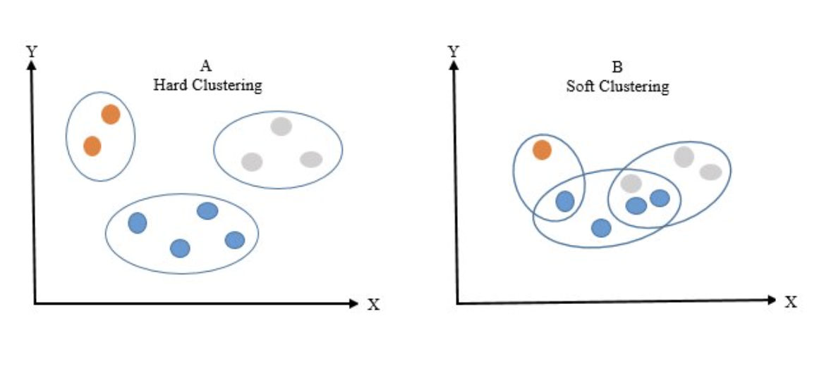
2.1 Hard vs. Soft Clustering

Hard Clustering: Assigns each data point to exactly one cluster.
- Use Cases: Market segmentation, customer grouping, and document clustering.
- Limitation: Cannot handle overlapping groups where a point might logically belong to multiple clusters.
Soft Clustering: Allows a data point to belong to multiple clusters simultaneously, utilizing probabilities (e.g., 70% in Cluster 1, 30% in Cluster 2).
- Use Cases: Overlapping class boundaries, customer personas, and medical diagnosis.
- Benefits: Captures ambiguity when boundaries are unclear.

2.2 K-Means Algorithm

2.2.1 Introduction

K-Means groups points based on their distance to cluster centers to identify natural groupings in raw, unorganized data.

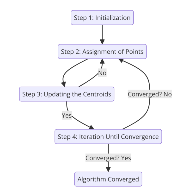
The Algorithm Steps:

Initialization: Randomly choose initial centroids from the data points.
Assignment: Assign each data point to the nearest centroid to form clusters.
Update Centroids: Recalculate the centroids by finding the mean of the points currently in each cluster.
Convergence: Repeat the assignment and update steps until the centroids stabilize and stop moving.

2.2.2 Advantages & Disadvantages

Advantages

It is fast, highly scalable for large datasets, easy to interpret, and highly efficient for well-separated, spherical data.

Disadvantages

It is highly sensitive to outliers, requires manually predefining the number of clusters k, and struggles with complex, non-convex shapes.

2.2.3 Getting the optimal k

The elbow method is used to find the optimal number of clusters k by plotting the Within-Cluster Sum of Squares (WCSS) against different k values.

$$WCSS = \sum_{i=1}^{k}\sum_{j=1}^{n_i}\left\lVert \mathbf{x}_j^{(i)} - \mathbf{c}_i \right\rVert^2 \tag{1}$$

Where:

i = 1,...,k: Iterates over all k clusters.
j = 1,...,n_i: Iterates over the n_i data points assigned to cluster i.
x_j⁽ⁱ⁾: The j^th data point belonging to cluster i.
c_i: The centroid (mean or center) of cluster i.
‖x_j⁽ⁱ⁾ − c_i‖²: The squared Euclidean distance between a data point and its corresponding cluster centroid.
WCSS: The total Within-Cluster Sum of Squares, representing the overall compactness of all clusters.

The Within-Cluster Sum of Squares (WCSS) measures the total squared distance between each data point and the centroid of the cluster to which it belongs. A lower WCSS indicates that data points are more tightly grouped around their centroids, implying more compact and cohesive clusters. In the Elbow Method, WCSS is computed for different values of k, and the optimal number of clusters is typically chosen at the point where further increases in k produce only marginal reductions in WCSS. Two major metrics are commonly used in the Elbow Method to evaluate clustering quality.

Distortion: Measures the average squared distance between each data point and its assigned cluster centroid. It quantifies how well the clusters represent the data. Lower distortion values indicate more compact clusters.

$$Distortion = \frac{1}{n}\sum_{i=1}^{n} \min_{c_j \in C} \left\lVert \mathbf{x}_i - \mathbf{c}_j \right\rVert^2 \tag{2}$$

Inertia (Within-Cluster Sum of Squares): Represents the sum of squared distances from each data point to the centroid of its assigned cluster. It is the optimization objective minimized by the K-Means algorithm.

$$Inertia = \sum_{i=1}^{k}\sum_{j=1}^{n_i}\left\lVert \mathbf{x}_j^{(i)} - \mathbf{c}_i \right\rVert^2 \tag{3}$$

2.3 Hierarchical Clustering

2.3.1 Introduction

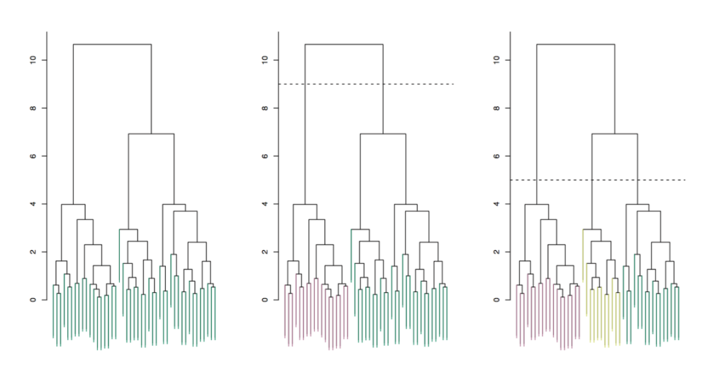
This technique groups data into a hierarchy of clusters based on similarity, visualizing relationships through a tree-like structure called a dendrogram.

Dendrogram: Each leaf in a dendrogram is a sample/ observation. As we move up the dendrogram, observations that are similar to each other begin to fuse into branches. Branches then fuse into bigger branches. Observations that fuse later (near the top of the tree, or root) are more different than observations that fuse earlier
Clusters: Clusters are created by making a horizontal cut across the dendrogram. Clusters are the separate trees below the cut.

Figure 3: Cluster creation using a dendrogram

2.3.2 Types of Hierarchical Clustering

Agglomerative (Bottom-Up)

Starts with every data point as a single cluster and successively merges pairs until all data is in one giant cluster.

Divisive (Top-Down)

Starts with all data in a single cluster and recursively splits them until each point is its own singleton cluster.

2.3.3 Types of Linkages

Single Linkage: Measures the distance between the two closest points in the respective clusters.
Complete Linkage: Measures the distance between the two furthest points in the respective clusters.
Average Linkage: Measures the average distance between all possible pairs of points across the two clusters. Ward's Linkage: Merges clusters to minimize the increase in total within-cluster variance (Sum of Squared Errors, or SSE).

2.4 DBSCAN (Density-Based Spatial Clustering of Applications with Noise)

2.4.1 Introduction

DBSCAN is a density-based clustering algorithm that groups data points that are closely packed together and marks outliers as noise based on their density in the feature space. It identifies clusters as dense regions in the data space separated by areas of lower density.

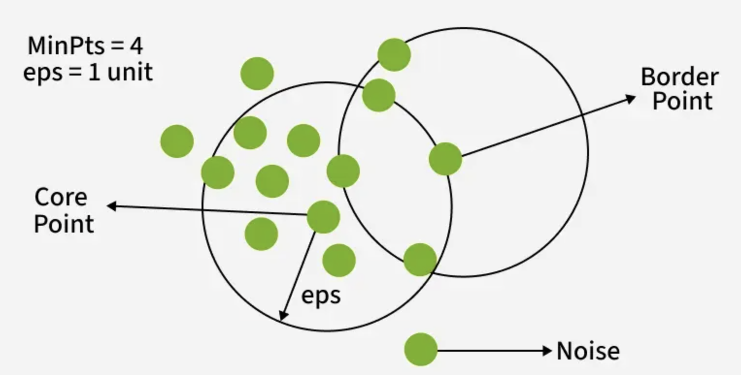
2.4.2 Key Parameters in DBSCAN

eps: This defines the radius of the neighborhood around a data point. If the distance between two points is less than or equal to eps they are considered neighbors. Choosing the right eps is important:
- If eps is too small most points will be classified as noise.
- If eps is too large, clusters may merge and the algorithm may fail to distinguish between them.
MinPts: This is the minimum number of points required within the eps radius to form a dense region.

3 Dimensionality Reduction

Dimensionality reduction is used in reducing the total feature count while preserving the underlying variance and structure of the data. It helps eliminate collinearity, accelerates model training, and allows data visualization in 2D or 3D.

3.1 Principal Component Analysis (PCA)

3.1.1 Introduction

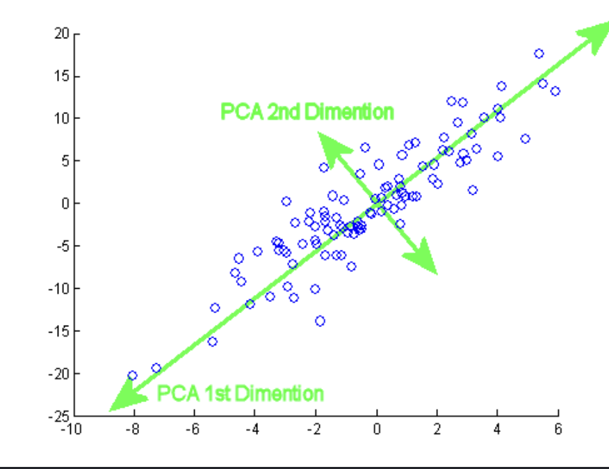
PCA is a linear technique that projects data onto new orthogonal axes called Principal Components. The first component captures the absolute maximum variance, and each subsequent component captures the remaining variance while staying perfectly perpendicular to the previous one.

Principal components (PC1 against PC2) — Figure 5: Pricipal components(PC1 against PC2)

3.1.2 PCA Implementation

Principal Component Analysis (PCA) transforms a high-dimensional dataset into a lower-dimensional representation while preserving as much of the original variance as possible. The implementation consists of the following steps.

Step 1: Standardize the Data

Since the variables in a dataset may have different units and scales, PCA begins by standardizing each feature so that they have a mean of zero and a standard deviation of one. The sample mean of a variable is computed as

$$\bar{X} = \frac{1}{n}\sum_{i=1}^{n} X_i,$$

while the sample variance is given by

$$\sigma^2 = \frac{1}{n-1}\sum_{i=1}^{n} (X_i - \bar{X})^2.$$

Each feature is then standardized using

$$Z = \frac{X - \bar{X}}{\sigma},$$

where X is the original variable, X̄ is its mean, and σ is its standard deviation. After standardization, each variable has a mean of 0 and a standard deviation of 1, ensuring that no feature dominates the analysis because of its scale.

Step 2: Compute the Covariance Matrix

Once the data have been standardized, the relationships between variables are summarized using the covariance matrix. The covariance between two variables X_i and X_j is computed as

$$Cov(X_i,X_j) = \frac{1}{n-1}\sum_{k=1}^{n} (X_i^{(k)} - \bar{X}_i)(X_j^{(k)} - \bar{X}_j).$$

In matrix form, the covariance matrix is expressed as

$$S = \frac{1}{n-1} X^{T}X,$$

where X is the standardized data matrix of size n × p, and S is the resulting p × p covariance matrix. Each element of the covariance matrix is

$$s_{ij} = \frac{1}{n-1}\sum_{k=1}^{n} x_{k,i}x_{k,j},$$

where x_k,i and x_k,j denote the standardized values of variables i and j for the k^th observation. The covariance matrix is always square, symmetric, and positive semi-definite.

Step 3: Compute the Eigenvalues and Eigenvectors

The principal components are obtained by computing the eigenvalues and eigenvectors of the covariance matrix. Let S denote the covariance matrix. The eigenvalue problem is defined as

$$Sv = \lambda v,$$

where

λ is an eigenvalue representing the amount of variance explained by a principal component.
v is the corresponding eigenvector representing the direction of maximum variance.

The eigenvalues are obtained by solving the characteristic equation

$$\det(S - \lambda I) = 0,$$

where I is the identity matrix. Each eigenvalue has an associated eigenvector, and together they define the new orthogonal feature space.

Step 4: Select the Principal Components

The eigenvalues are sorted in descending order according to the amount of variance they explain. The explained variance ratio for the i^th principal component is

$$\text{Explained Variance Ratio} = \frac{\lambda_i}{\sum_{j=1}^{p} \lambda_j}.$$

The cumulative explained variance is then computed to determine how many principal components should be retained. A common practice is to select the smallest number of principal components that preserve at least 95% of the total variance. For visualization purposes, the first two principal components (PC1 and PC2) are often selected because they capture the largest proportion of the dataset's variability.

Step 5: Project the Data onto the New Feature Space

Finally, the standardized data are projected onto the selected principal components to obtain a lower-dimensional representation. If W contains the selected eigenvectors, the transformed data are computed as

$$Y = XW,$$

where

X is the standardized data matrix,
W is the projection matrix formed from the selected eigenvectors,
Y is the reduced-dimensional representation of the original dataset.

The transformed dataset can then be used for visualization, clustering, classification, or as a preprocessing step for other machine learning algorithms.

3.1.3 Advantages and Disadvantages

Advantages

Handles multicollinearity (creates uncorrelated variables), reduces noise, compresses data for faster processing, and aids in outlier detection.

Disadvantages

The new components can be difficult to interpret, it is highly sensitive to proper data scaling, some important information may be lost, it assumes linearity in the data, and it is computationally heavy for massive datasets.

3.2 Non-Negative Matrix Factorization (NMF)

Non-Negative Matrix Factorization (NMF) is a dimensionality reduction technique that decomposes a non-negative data matrix into two lower-dimensional non-negative matrices. Because all values remain non-negative, the learned representations are often more interpretable than those produced by PCA.

Given a non-negative matrix

$$A \in \mathbb{R}^{m \times n}, \quad A_{ij} \geq 0,$$

NMF approximates the matrix as

$$A_{m \times n} \approx W_{m \times k}H_{k \times n},$$

where

A is the original data matrix,
W contains the basis (feature) vectors,
H contains the coefficients or encoding of each sample,
k is the reduced dimensionality with k ≪ min(m,n).

4 Anomaly Detection using DBSCAN

Density-Based Spatial Clustering of Applications with Noise (DBSCAN) is one of the most effective clustering algorithms for anomaly detection because it naturally identifies isolated observations as noise. Unlike K-Means, which forces every data point into a cluster, DBSCAN groups together points located in high-density regions while treating sparse regions as anomalies.

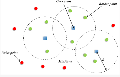
A point is assigned to a cluster if it has at least MinPts neighboring points within a specified radius (ε). Based on this criterion, DBSCAN categorizes observations into three groups:

Core Points: Points having at least MinPts neighbors within radius ε.
Border Points: Points that lie within the neighborhood of a core point but have fewer than MinPts neighbors themselves.
Noise (Outlier) Points: Points that are neither core nor border points and are considered anomalies.

Anomaly detection: core points, border points, and noise points identified by DBSCAN — Figure 6: Anomaly detection

Because DBSCAN does not force every observation into a cluster, isolated points in low-density regions are naturally labeled as Noise, making the algorithm particularly suitable for anomaly detection in applications such as fraud detection.

Practical

Put clustering, dimensionality reduction, and anomaly detection into practice in the guided Colab notebook below.

Open the practical notebook ↗

References

For more information, visit: