Hydrology Graph Neural Networks PyTorch Geometric GIS

Graph Neural Networks for Hydrological Spatial Imputation

By Bethwel Rotich · ~15 min read

Introduction

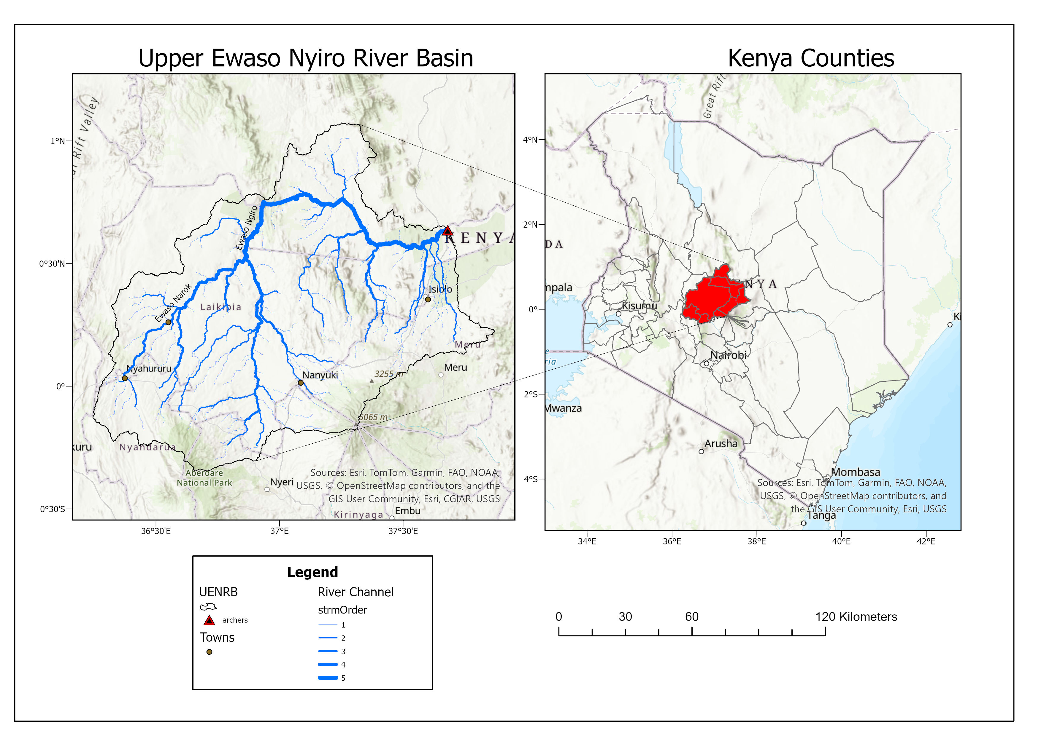
Hydrology is the study of water movement, distribution, and storage across the landscape. At the basin scale, a river basin is the area of land that drains into a common outlet, and hydrological processes are strongly shaped by physical connectivity between upstream and downstream sub-basins.

In real-world hydrological monitoring, streamflow monitoring stations (stream gauges) are often sparse, malfunctioning, or unevenly distributed. This tutorial shows how hydrological river systems can be modeled as graph-structured data, where directional flow relationships and spatial topology are preserved to perform spatial streamflow imputation using Graph Convolutional Networks (GCN).

Get the complete GNN_HYDROLOGY.ipynb Jupyter Notebook and follow along.

Download Notebook (.ipynb)

What is a Graph?

A graph $G = (V, E)$ is a fundamental data structure composed of:

Nodes (Vertices, $V$)

Represent entities in the domain (e.g., individual sub-basins, water gauges, or weather stations).

Edges (Links, $E$)

Represent connections or functional relationships between nodes (e.g., physical river flow channels connecting upstream sub-basins to downstream ones).

Types of Graphs in Spatial Modeling

Graphs can be undirected (bidirectional connections) or directed (one-way relationships, such as water flowing downstream). Edges can also be weighted (e.g., length of river segment or channel capacity) or unweighted.

Why Do We Need Graphs in Hydrology?

In geographic information systems (GIS), topology describes the relative location and connectivity of spatial features independent of their exact geometry.

Hydrological systems present unique challenges:

Spatially connected: Upstream rainfall directly drives downstream discharge.
Temporally dynamic: Rainfall-runoff impacts experience propagation delays along river channels.
Nonlinear interactions: Soil moisture, slope, and land use create complex non-linear discharge behaviors.

Limitation of Traditional ML Models

Standard Machine Learning models (like Random Forests or MLPs) treat spatial locations as independent samples or oversimplify spatial relationships into Euclidean distances, ignoring directional water routing. Graph Neural Networks explicitly preserve river routing topology.

Environment & Package Setup

To build GNNs for hydrological applications, we require PyTorch, PyTorch Geometric (`torch_geometric`), GeoPandas for vector GIS data, and Xarray for NetCDF hydrological discharge grid handling.

Python

# Install PyTorch Geometric and geospatial dependencies
!pip install -q torch-geometric geopandas xarray netCDF4 networkx matplotlib scipy scikit-learn

import os
import torch
import torch.nn as nn
import torch.nn.functional as F
from torch_geometric.nn import GCNConv
from torch_geometric.utils import dense_to_sparse
from torch_geometric.data import Data
import geopandas as gpd
import xarray as xr
import numpy as np
import networkx as nx
import matplotlib.pyplot as plt
from sklearn.metrics import mean_squared_error, mean_absolute_error, r2_score

print(f"PyTorch Version: {torch.__version__}")

Loading & Preprocessing Sub-basin Shapefiles

We use HydroSHEDS / HydroBASINS shapefile polygon layers representing catchment boundaries. Each sub-basin has a unique identifier (`HYBAS_ID`) and a downstream target ID (`NEXT_DOWN`), which defines the physical flow directional graph.

Python

# Load sub-basins shapefile
shapefile_path = "hydrobasins_layer.shp" # Update to your local path
hydrobasins = gpd.read_file(shapefile_path)

# Filter sub-basins within the region of interest
# Ensure attributes HYBAS_ID and NEXT_DOWN are present
print(f"Total sub-basins loaded: {len(hydrobasins)}")
print(hydrobasins[['HYBAS_ID', 'NEXT_DOWN', 'SUB_AREA']].head())

Constructing the Basin Directed Adjacency Matrix ($A$)

We convert the spatial topology into a binary adjacency matrix $A \in \mathbb{R}^{N \times N}$, where $A_{ij} = 1$ indicates a river flow connection from sub-basin $i$ to sub-basin $j$.

Python

# Create mapping from HYBAS_ID to matrix index
nodes = hydrobasins_filtered['HYBAS_ID'].tolist()
id_to_idx = {hybas_id: idx for idx, hybas_id in enumerate(nodes)}

N = len(nodes)
A = np.zeros((N, N), dtype=np.float32)

# Build directed edges based on NEXT_DOWN flow direction
for _, row in hydrobasins_filtered.iterrows():
    u_id = row['HYBAS_ID']
    v_id = row['NEXT_DOWN']
    if u_id in id_to_idx and v_id in id_to_idx:
        u_idx = id_to_idx[u_id]
        v_idx = id_to_idx[v_id]
        A[u_idx, v_idx] = 1.0  # Directed edge: u flows into v

print(f"Adjacency Matrix constructed for {N} sub-basins.")
print(f"Total Directed River Connections (Edges): {int(A.sum())}")

Visualizing the Hydrological Basin Graph

We can map sub-basin centroids and draw directed edges representing water flow across the basin network using `NetworkX`.

Python

# Compute centroid positions for plotting
centroids = {
    row["HYBAS_ID"]: (row.geometry.centroid.x, row.geometry.centroid.y)
    for _, row in hydrobasins_filtered.iterrows()
}

G = nx.DiGraph()
for hybas_id in nodes:
    G.add_node(hybas_id)

for u_id in nodes:
    v_id = hydrobasins_filtered.loc[hydrobasins_filtered['HYBAS_ID'] == u_id, 'NEXT_DOWN'].values[0]
    if v_id in id_to_idx:
        G.add_edge(u_id, v_id)

pos = {node: centroids[node] for node in G.nodes()}

fig, ax = plt.subplots(figsize=(10, 8))
hydrobasins_filtered.plot(ax=ax, facecolor='none', edgecolor='lightgray', linewidth=0.8)
nx.draw_networkx_nodes(G, pos=pos, ax=ax, node_size=30, node_color='teal')
nx.draw_networkx_edges(G, pos=pos, ax=ax, edge_color='red', arrows=True, arrowsize=10, width=1.2)

plt.title("Hydrological Sub-basin Directed Flow Network", fontsize=14, fontweight='bold')
plt.xlabel("Longitude")
plt.ylabel("Latitude")
plt.show()

Loading Discharge Telemetry & Temporal Lags

We load GloFAS (Global Flood Awareness System) reanalysis daily discharge NetCDF datasets using `xarray`. To capture temporal wave propagation, we calculate historical lagged discharge features (e.g., 1-day, 2-day, 3-day lags).

Python

nc_path = "glofas_reanalysis_2025_12.nc" # Path to NetCDF file
ds = xr.open_dataset(nc_path)
DIS_VAR = "dis24" # 24-hour accumulated streamflow discharge

LAG_DAYS = [1, 2, 3]
TIME_IDX = max(LAG_DAYS) # Time snapshot index

# Extract discharge values per sub-basin centroid
discharge_values = []
for hybas_id in nodes:
    lon, lat = centroids[hybas_id]
    val = ds[DIS_VAR].isel(valid_time=TIME_IDX).sel(
        latitude=lat, longitude=lon, method="nearest"
    ).values.item()
    discharge_values.append(val)

discharge_values = np.array(discharge_values, dtype=np.float32)

# Handle NaNs by mean replacement & Z-score normalization
nan_mask = np.isnan(discharge_values)
if nan_mask.any():
    discharge_values[nan_mask] = np.nanmean(discharge_values)

x_raw = torch.tensor(discharge_values, dtype=torch.float32).unsqueeze(1)
x_mean, x_std = x_raw.mean(), x_raw.std() + 1e-8
x_norm = (x_raw - x_mean) / x_std

Data Masking for Spatial Imputation Task

To simulate unmonitored or broken stream gauges, we partition the sub-basins into **Training (60%)**, **Validation (20%)**, and **Test (20%)** sets. For validation and test sub-basins, current discharge values are zero-masked ($0.0$) in `data.x`, and the GNN model must infer them based on graph connectivity and lagged discharge context!

Python

# Convert Adjacency matrix into PyTorch Sparse Tensor COO Format
A_tensor = torch.tensor(A, dtype=torch.float32)
edge_index, edge_weight = dense_to_sparse(A_tensor)

# Generate train/val/test split masks
torch.manual_seed(42)
n_nodes = x_norm.shape[0]
shuffled_indices = torch.randperm(n_nodes)

n_test = int(0.20 * n_nodes)
n_val = int(0.20 * n_nodes)
n_train = n_nodes - n_test - n_val

train_mask = torch.zeros(n_nodes, dtype=torch.bool)
val_mask = torch.zeros(n_nodes, dtype=torch.bool)
test_mask = torch.zeros(n_nodes, dtype=torch.bool)

train_mask[shuffled_indices[n_test + n_val:]] = True
val_mask[shuffled_indices[n_test : n_test + n_val]] = True
test_mask[shuffled_indices[:n_test]] = True

# Construct PyTorch Geometric Data Object
data = Data(x=x_norm.clone(), edge_index=edge_index, y=x_norm.clone())
data.train_mask = train_mask
data.val_mask = val_mask
data.test_mask = test_mask

# Apply zero-masking to validation & test target features in input data.x
data.x[data.val_mask, 0] = 0.0
data.x[data.test_mask, 0] = 0.0

print(f"Graph Data Object: {data}")
print(f"Train nodes: {train_mask.sum().item()}, Val nodes: {val_mask.sum().item()}, Test nodes: {test_mask.sum().item()}")

Spatial GCN Model Architecture

We implement a multi-layer Graph Convolutional Network (`SpatialGCN`) using `GCNConv` layers. Graph convolution updates a node's state by aggregating normalized representations from neighboring upstream/downstream sub-basins:

$$H^{(l+1)} = \sigma \left( \tilde{D}^{-\frac{1}{2}} \tilde{A} \tilde{D}^{-\frac{1}{2}} H^{(l)} W^{(l)} \right)$$

Python

class SpatialGCN(nn.Module):
    """
    Graph Convolutional Network for Hydrological Spatial Streamflow Imputation.
    """
    def __init__(self, in_ch, hidden, out_ch, dropout_rate, num_layers, activation_fn=F.leaky_relu):
        super().__init__()
        self.num_layers = num_layers
        self.dropout = nn.Dropout(p=dropout_rate)
        self.activation_fn = activation_fn

        self.conv_layers = nn.ModuleList()
        self.bn_layers = nn.ModuleList()

        # Input GCN Layer
        self.conv_layers.append(GCNConv(in_ch, hidden))
        if num_layers > 1:
            self.bn_layers.append(nn.BatchNorm1d(hidden))

        # Hidden GCN Layers
        for _ in range(num_layers - 2):
            self.conv_layers.append(GCNConv(hidden, hidden))
            self.bn_layers.append(nn.BatchNorm1d(hidden))

        # Final Output Layer for continuous discharge regression
        if num_layers > 1:
            self.conv_layers.append(GCNConv(hidden, out_ch))

    def forward(self, x, edge_index):
        for i in range(self.num_layers - 1):
            x = self.conv_layers[i](x, edge_index)
            if len(self.bn_layers) > i:
                x = self.bn_layers[i](x)
            x = self.activation_fn(x)
            x = self.dropout(x)
        
        # Output layer (no activation for linear regression output)
        x = self.conv_layers[-1](x, edge_index)
        return x

Model Training & Optimization

We train the `SpatialGCN` model using Adam optimizer, Mean Squared Error (MSE) loss on training nodes, and dynamic learning rate reduction (`ReduceLROnPlateau`).

Python

# Instantiate model hyperparameters
torch.manual_seed(42)
model = SpatialGCN(
    in_ch=data.x.shape[1],
    hidden=16,
    out_ch=1,
    dropout_rate=0.4,
    num_layers=2,
    activation_fn=F.leaky_relu
)

optimizer = torch.optim.Adam(model.parameters(), lr=0.0025, weight_decay=1e-3)
loss_fn = nn.MSELoss()
scheduler = torch.optim.lr_scheduler.ReduceLROnPlateau(optimizer, mode='min', factor=0.5, patience=20)

epochs = 300
for epoch in range(1, epochs + 1):
    model.train()
    optimizer.zero_grad()
    
    out = model(data.x, data.edge_index)
    loss = loss_fn(out[data.train_mask], data.y[data.train_mask])
    
    loss.backward()
    optimizer.step()
    
    # Validation evaluation
    model.eval()
    with torch.no_grad():
        val_out = model(data.x, data.edge_index)
        val_loss = loss_fn(val_out[data.val_mask], data.y[data.val_mask])
        scheduler.step(val_loss)
        
    if epoch % 50 == 0:
        print(f"Epoch {epoch:03d} | Train MSE: {loss.item():.4f} | Val MSE: {val_loss.item():.4f}")

Evaluation & Results

We evaluate model performance on the held-out **test nodes** (which were completely masked during input formulation) using Mean Squared Error (MSE), Mean Absolute Error (MAE), and $R^2$ coefficient of determination.

Python

model.eval()
with torch.no_grad():
    test_preds = model(data.x, data.edge_index)[data.test_mask].squeeze().cpu().numpy()
    test_trues = data.y[data.test_mask].squeeze().cpu().numpy()

mse = mean_squared_error(test_trues, test_preds)
mae = mean_absolute_error(test_trues, test_preds)
r2 = r2_score(test_trues, test_preds)

print("--- Test Set Imputation Evaluation ---")
print(f"Test MSE : {mse:.4f}")
print(f"Test MAE : {mae:.4f}")
print(f"Test R²  : {r2:.4f}")

# Plotting Predictions vs Ground Truth
plt.figure(figsize=(7, 6))
plt.scatter(test_trues, test_preds, alpha=0.8, color='teal', label='Unmonitored Sub-basins')
plt.plot([min(test_trues), max(test_trues)], [min(test_trues), max(test_trues)], 'r--', label='1:1 Perfect Line')
plt.title("Spatial Streamflow Imputation: Actual vs Predicted", fontsize=12, fontweight='bold')
plt.xlabel("True Normalized Discharge")
plt.ylabel("Predicted Normalized Discharge")
plt.legend()
plt.grid(True, linestyle='--', alpha=0.5)
plt.show()

Key Conclusion

By integrating river network topology via PyTorch Geometric GCNs and temporal lagged streamflow features, the model effectively reconstructs missing streamflow telemetry across unmonitored river basins with high $R^2$ accuracy.

References

Zhou, J., et al. (2020). Graph neural networks: A review of methods and applications. AI Open, 1, 57–81.
Mosaffa, H., et al. (2026). A GNN routing module is all you need for LSTM Rainfall–Runoff models. Hydrology and Earth System Sciences, 30(7), 2079–2092.

Bethwel Rotich

Table of Contents

Table of Contents

Graph Neural Networks for Hydrological Spatial Imputation

Introduction

What is a Graph?

Nodes (Vertices, $V$)

Edges (Links, $E$)

Why Do We Need Graphs in Hydrology?

Environment & Package Setup

Loading & Preprocessing Sub-basin Shapefiles

Constructing the Basin Directed Adjacency Matrix ($A$)

Visualizing the Hydrological Basin Graph

Loading Discharge Telemetry & Temporal Lags

Data Masking for Spatial Imputation Task

Spatial GCN Model Architecture

Model Training & Optimization

Evaluation & Results

References

Bethwel Rotich

Table of Contents

Table of Contents

Introduction

What is a Graph?

Nodes (Vertices, $V$)

Edges (Links, $E$)

Why Do We Need Graphs in Hydrology?

Environment & Package Setup

Loading & Preprocessing Sub-basin Shapefiles

Constructing the Basin Directed Adjacency Matrix ($A$)

Visualizing the Hydrological Basin Graph

Loading Discharge Telemetry & Temporal Lags

Data Masking for Spatial Imputation Task

Spatial GCN Model Architecture

Model Training & Optimization

Evaluation & Results

References

Related Tutorials

Introduction to Depth Anything V2

Introduction to NLP