Computer Vision AI Forestry

From Flat Pixels to 3D Spaces: An Introduction to Depth Anything V2

By Samuel Mbatia · 4 May, 2026 · ~12 min read

Depth Anything V2 — official teaser showing depth estimation results

Introduction

Today, we are going to teach a computer how to see depth in a standard, 2D photograph.

Whether you are analysing the structure of a forest canopy from an RGB drone image or helping a robot navigate a room, understanding the physical distance of objects without expensive 3D sensors is one of the biggest challenges in computer vision.

Let's look at how Monocular Depth Estimation (MDE) solves this — and then apply it to a real forestry use case.

Get the complete DepthAnythingV2.ipynb and follow along at your own pace.

Download (.ipynb)

Enter Depth Anything V2

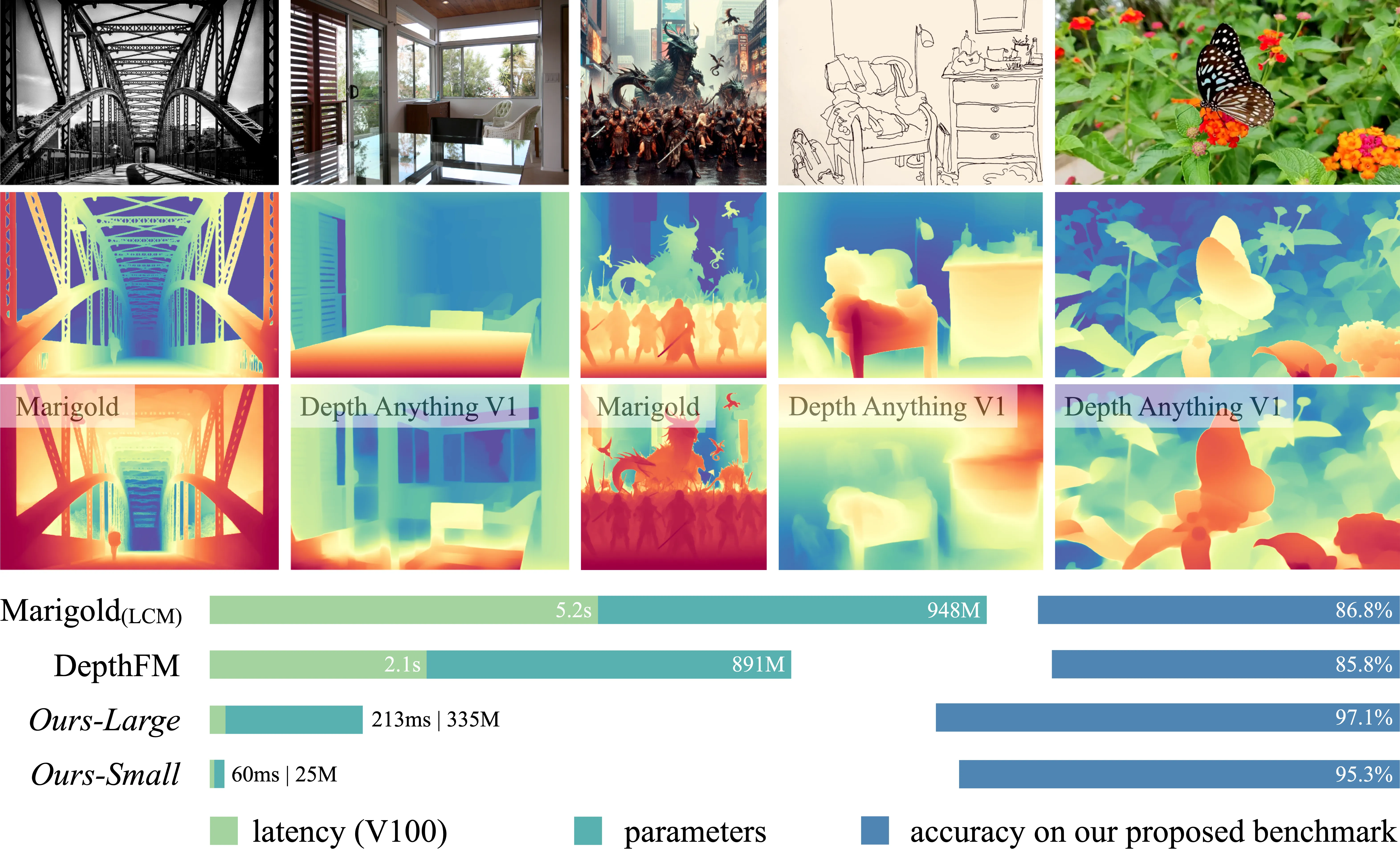
Released in 2024, Depth Anything V2 is a “foundation model” built specifically to estimate depth flawlessly across any environment.

How is it so accurate? The Teacher-Student Method:

The Teacher: Researchers trained a massive AI on 595,000 perfectly accurate synthetic (computer-generated) 3D images.
The Massive Dataset: This Teacher AI then labelled over 62 million real-world, unlabelled images.
The Student: Those 62 million images were used to train the efficient “Student” models we use today.

The result? Unmatched detail — capturing incredibly fine features like thin branches and sharp edges — running 10× faster than previous models.

Setting Up

We start by mounting Google Drive and installing the required libraries.

Python

# Mount Google Drive (Google Colab only)
from google.colab import drive
drive.mount('/content/drive')

Python

# Install required libraries
!pip install transformers huggingface_hub pillow matplotlib rasterio

from PIL import Image
import matplotlib.pyplot as plt
from transformers import pipeline

print("Libraries loaded successfully!")

Python

print("Downloading and loading the Depth Anything V2 model...")

# Hugging Face pipeline abstracts away the complex architecture.
# The 'Small' version is fast enough for standard hardware.
pipe = pipeline(task="depth-estimation", model="depth-anything/Depth-Anything-V2-Small-hf")

print("Model loaded and ready!")

The Stress Test

We use an RGB aerial image of a forest. This is a fantastic stress test: the model must figure out the structural complexity of overlapping tree crowns and the ground below.

Python

image_path = '/content/drive/MyDrive/DepthAnything/images/semi_urban.jpg'
image = Image.open(image_path)

# THE MAGIC: one line extracts depth
result = pipe(image)
depth_map = result["depth"]

# Side-by-side plot
fig, axes = plt.subplots(1, 2, figsize=(16, 8))
axes[0].imshow(image)
axes[0].set_title("Original RGB Image", fontsize=14)
axes[0].axis("off")

# Brighter = closer/higher, darker = further/lower
axes[1].imshow(depth_map, cmap='inferno')
axes[1].set_title("Predicted Depth Map (Depth Anything V2)", fontsize=14)
axes[1].axis("off")

plt.tight_layout()
plt.show()

You can also loop over an entire folder of images and process them in batch:

Python

import os, glob

folder_path = '/content/drive/MyDrive/DepthAnything/images'
image_files = glob.glob(f"{folder_path}/*.[jp][pn]*")

for img_path in image_files:
    file_name = os.path.basename(img_path)
    image = Image.open(img_path)
    result = pipe(image)
    depth_map = result["depth"]

    fig, axes = plt.subplots(1, 2, figsize=(15, 6))
    axes[0].imshow(image)
    axes[0].set_title(f"Original RGB: {file_name}", fontsize=12)
    axes[0].axis("off")
    axes[1].imshow(depth_map, cmap='inferno')
    axes[1].set_title("Predicted Depth Map", fontsize=12)
    axes[1].axis("off")
    plt.tight_layout()
    plt.show()

Application in Forestry

Drone surveys of forests produce hundreds of georeferenced .tif image tiles. We can run Depth Anything V2 on each tile to produce a relative depth map, then stitch those maps into a single unified spatial mosaic. Access the sample data via the Technical Session Folder.

Python

import rasterio
from rasterio.plot import show

tile1_path = "/content/drive/MyDrive/Data Preview/tiles/2024_08_386.tif"
tile2_path = "/content/drive/MyDrive/Data Preview/tiles/2024_08_385.tif"

fig, (ax1, ax2) = plt.subplots(1, 2, figsize=(14, 7))
with rasterio.open(tile1_path) as src1, rasterio.open(tile2_path) as src2:
    show(src1, ax=ax1, title="Sample Tile One")
    show(src2, ax=ax2, title="Sample Tile Two")
plt.show()

Geospatial Mosaicing

Because drone surveys are made of hundreds of overlapping tiles, we need to stitch our predicted depth maps together to see the entire surveyed area. Since we combine the AI output with rasterio, the depth maps automatically inherit the geographic metadata (CRS and spatial transforms) of the original .tif tiles.

Python

import numpy as np
from rasterio.merge import merge

tile_paths = [tile1_path, tile2_path]
temp_depth_files = []

for i, path in enumerate(tile_paths):
    with rasterio.open(path) as src:
        meta = src.meta.copy()
        img_array = src.read([1, 2, 3])
        img_array = np.transpose(img_array, (1, 2, 0))
        pil_image = Image.fromarray(img_array)

        result = pipe(pil_image)
        relative_depth = np.array(result["depth"], dtype=np.float32)

        meta.update(count=1, dtype='float32')
        out_path = f"temp_depth_tile_{i}.tif"
        with rasterio.open(out_path, 'w', **meta) as dest:
            dest.write(relative_depth, 1)
        temp_depth_files.append(out_path)

# Merge tiles into a single mosaic
src_files_to_mosaic = [rasterio.open(fp) for fp in temp_depth_files]
mosaic, out_trans = merge(src_files_to_mosaic)
for src in src_files_to_mosaic:
    src.close()

im = plt.imshow(mosaic[0], cmap='inferno')
plt.colorbar(im, label="Relative Depth / Structure Intensity (0-255)", shrink=0.5)
plt.title("Merged Relative Depth Mosaic", fontsize=16)
plt.axis("off")
plt.show()

for fp in temp_depth_files:
    os.remove(fp)

Ground Truthing: Calibrating AI to Reality

The depth map above is relative — pixel values range from 0 to 255, not real-world metres. To extract true scientific value (like estimating above-ground biomass) we need absolute metric heights.

We do this by:

Extracting the AI’s predicted 0–255 value at the exact GPS coordinate of every field-measured tree.
Comparing the AI’s guess to the true field measurement.
Using Linear Regression to derive a formula that converts any AI pixel into true metres.

Python

import geopandas as gpd
from rasterio.transform import rowcol
from scipy.stats import linregress

shp_path = "/content/drive/MyDrive/DepthAnything/Technicalssession/Shapefile/Groundtruthfielddata.shp"
trees_gdf = gpd.read_file(shp_path)

# Align CRS with our mosaic
with rasterio.open(tile_paths[0]) as src_crs_check:
    mosaic_crs = src_crs_check.crs
if trees_gdf.crs != mosaic_crs:
    trees_gdf = trees_gdf.to_crs(mosaic_crs)

# Convert GPS coords to pixel rows/columns
xs = trees_gdf.geometry.x.values
ys = trees_gdf.geometry.y.values
rows, cols = rowcol(out_trans, xs, ys)

# Sample AI values at each tree location
ai_values = []
for r, c in zip(rows, cols):
    if 0 <= r < mosaic.shape[1] and 0 <= c < mosaic.shape[2]:
        ai_values.append(mosaic[0, r, c])
    else:
        ai_values.append(float('nan'))

trees_gdf['ai_relative'] = ai_values
trees_gdf['height_m'] = trees_gdf['TH__cm_'] / 100

clean_df = trees_gdf.dropna(subset=['ai_relative', 'height_m'])
slope, intercept, r_value, p_value, std_err = linregress(clean_df['ai_relative'], clean_df['height_m'])

print(f"Formula: True Height(m) = ({slope:.6f} * AI_Value) + {intercept:.4f}")
print(f"R\u00b2 Accuracy: {r_value**2:.4f}")

Mapping True Metric Height

Now that we have our calibration formula, we apply it to the entire surveyed area. By running every pixel through (Slope × Pixel_Value) + Intercept, we convert the abstract AI representation into a true Canopy Height Model (CHM). The colours you see represent actual metres above the ground.

Python

# Apply regression formula to the entire mosaic
metric_height_map = (mosaic[0] * slope) + intercept

# Clip negative values to 0 (trees can't have negative height)
metric_height_map = np.clip(metric_height_map, a_min=0, a_max=None)

# Compute geographic extent from the spatial transform
map_height, map_width = metric_height_map.shape
left   = out_trans.c
top    = out_trans.f
right  = left + (out_trans.a * map_width)
bottom = top  + (out_trans.e * map_height)
geographic_extent = [left, right, bottom, top]

fig, ax = plt.subplots(figsize=(14, 10))
im = ax.imshow(metric_height_map, cmap='viridis', extent=geographic_extent)
cbar = plt.colorbar(im, ax=ax, shrink=0.5)
cbar.set_label("True Canopy Height (Meters)", fontsize=14, fontweight='bold')

# Overlay GPS field measurement points
trees_gdf.plot(ax=ax, facecolor='red', edgecolor='white', markersize=60, marker='.', label='GPS Field Measurements')

plt.title("Final Calibrated Canopy Height Model (CHM)", fontsize=18, fontweight='bold')
plt.xlabel("Longitude / Easting", fontsize=12)
plt.ylabel("Latitude / Northing", fontsize=12)
plt.legend(loc='upper right', fontsize=12)
plt.tight_layout()
plt.show()

Samuel Mbatia

Table of Contents

Table of Contents

From Flat Pixels to 3D Spaces: An Introduction to Depth Anything V2

Introduction

Enter Depth Anything V2

Setting Up

The Stress Test

Application in Forestry

Geospatial Mosaicing

Ground Truthing: Calibrating AI to Reality

Mapping True Metric Height

Samuel Mbatia

Table of Contents

Table of Contents

Introduction

Enter Depth Anything V2

Setting Up

The Stress Test

Application in Forestry

Geospatial Mosaicing

Ground Truthing: Calibrating AI to Reality

Mapping True Metric Height

Related Articles

Introduction to NLP

KENET CHUI GPU Cluster Launch