Hydrology Commercial Microwave Links pycomlink GIS

Introduction to CML Data Processing: The Po Valley (OpenRainER)

By Samuel Mbugua · ~20 min read

Introduction

Technical Session: Opportunistic Precipitation Sensing via Commercial Microwave Links

Welcome to this technical session! Today we will learn how to transform raw telecommunication signal attenuation (TSL and RSL) from cellular networks into high-resolution, path-averaged rainfall estimates.

We will use the OpenRainER testbed located in Italy's Po Valley (Cite: Covi et al. 2024). For a general review of CML rainfall monitoring, see Cite: Uijlenhoet et al. 2018.

Learning Objectives

Load and explore 2 months of CML, physical rain gauge, and grid radar datasets.
Understand the physical principles and math of opportunistic rainfall sensing.
Implement the core retrieval pipeline on a single CML path at 1-minute resolution.
Compare different Wet Antenna Attenuation (WAA) estimation models.
Validate CML rainfall estimates at the native 15-minute sampling interval of the rain gauges.
Simulate 15-minute legacy networks using the RAINLINK consensus algorithm and prove the Peak-Flattening temporal resolution gap.

Get the complete Intro_CML_Processing_Po_Valley.ipynb Jupyter Notebook and follow along.

Download Notebook (.ipynb)

Environment & Dependency Setup

This first cell checks whether you're running in Google Colab. If so, it installs the CML processing stack and clones the repository containing the Po Valley datasets and reference images.

Python

# ==============================================================================
# Google Colab & Dependency Setup
# Run this cell to install required libraries and download datasets when in Colab.
# ==============================================================================
import sys
import os

if 'google.colab' in sys.modules:
    print("Running in Google Colab! Setting up environment...")

    # Install required CML and spatial libraries
    print("Installing pycomlink, poligrain, and cartopy...")
    !pip install -q pycomlink poligrain cartopy

    # Clone repository to access datasets
    repo_url = "https://github.com/mbuguasamuelwambui/2026-08-03-CML_Processing.git"
    repo_name = "2026-08-03-CML_Processing"

    if not os.path.exists('data/cml/po_valley_cmls.nc'):
        print(f"Cloning dataset repository from {repo_url}...")
        os.system(f"rm -rf {repo_name} data images")
        os.system(f"git clone {repo_url}")

        # Copy data and images directories to the working path
        src_data = f"{repo_name}/data"
        src_images = f"{repo_name}/images"
        if os.path.exists(src_data):
            os.system(f"cp -r {src_data} ./")
        if os.path.exists(src_images):
            os.system(f"cp -r {src_images} ./")
            print("Datasets and images successfully imported to Colab workspace!")
else:
    print("Running locally. Assuming datasets are already present in the 'data/' directory.")

Step 1: Library Imports

First, let's import our CML processing engine (pycomlink), our spatial validation and mapping library (poligrain), and core scientific data stacks.

Python

import os
import sys
import numpy as np
import pandas as pd
import xarray as xr
import matplotlib.pyplot as plt

import poligrain as plg
import pycomlink as pycml

# Set default plot styling
plt.style.use('seaborn-v0_8-whitegrid')
print("Libraries successfully imported!")

Section 1: Load and Explore CML Data

We load a 2-month dataset of CML signal telemetry. The dataset also includes physical rain gauges and regional weather radar grids.

Step 1.1: Loading the Dataset

Choose which month you want to load:

"2021-01" for January
"2021-11" for November

Then, load the NetCDF files and print their structures.

Python

# Select month to process: "2021-01" or "2021-11"
selected_month = "2021-01"  # Edit this to "2021-11" to run for November!

print(f"Loading datasets for {selected_month}...")
ds_cmls_all = xr.open_dataset("data/cml/po_valley_cmls.nc")
ds_gauges_all = xr.open_dataset("data/gauges/po_valley_gauges.nc")

# Subset CML and Gauges to selected month and load to memory
ds_cmls = ds_cmls_all.sel(time=selected_month).load()
ds_gauges = ds_gauges_all.sel(time=selected_month).load()
ds_cmls_all.close()
ds_gauges_all.close()

# Load the corresponding Radar dataset
radar_file = f"data/radar/RADadj_{selected_month.replace('-', '')}.nc"
ds_radar = xr.open_dataset(radar_file).load()
ds_radar.close()

print("\n=== CML Dataset ===")
print(ds_cmls)
print("\n=== Rain Gauge Dataset ===")
print(ds_gauges)
print("\n=== Radar Dataset ===")
print(ds_radar)

Step 1.2: Standardize Coordinates and Spatial Projection

To perform accurate spatial math, we project the coordinates. We convert geographic longitude/latitude into the local flat Universal Transverse Mercator (UTM Zone 32N, EPSG:25832) projection.

Why do this?

Latitude and longitude are angles, not flat distances. Projected UTM coordinates allow calculating exact distances in meters.

Python

# Standardize coordinate and variable names across raw dataset formats
if 'longitude' in ds_gauges.coords:
    ds_gauges = ds_gauges.rename({'longitude': 'lon', 'latitude': 'lat'})
if 'rainfall_amount' in ds_radar.variables and 'R' not in ds_radar.variables:
    ds_radar = ds_radar.rename({'rainfall_amount': 'R'})

# Project coordinates for rain gauges
ds_gauges.coords["x"], ds_gauges.coords["y"] = plg.spatial.project_point_coordinates(
    ds_gauges.lon, ds_gauges.lat, "EPSG:25832"
)

# Project coordinates for CML tower coordinates (endpoints)
ds_cmls.coords["site_0_x"], ds_cmls.coords["site_0_y"] = plg.spatial.project_point_coordinates(
    ds_cmls.site_0_lon, ds_cmls.site_0_lat, "EPSG:25832"
)
ds_cmls.coords["site_1_x"], ds_cmls.coords["site_1_y"] = plg.spatial.project_point_coordinates(
    ds_cmls.site_1_lon, ds_cmls.site_1_lat, "EPSG:25832"
)

# Project coordinates for rectilinear radar grid
lon_grid, lat_grid = np.meshgrid(ds_radar.lon.values, ds_radar.lat.values)
lon_da = xr.DataArray(lon_grid, dims=('lat', 'lon'), coords={'lat': ds_radar.lat, 'lon': ds_radar.lon})
lat_da = xr.DataArray(lat_grid, dims=('lat', 'lon'), coords={'lat': ds_radar.lat, 'lon': ds_radar.lon})
x_grid, y_grid = plg.spatial.project_point_coordinates(lon_da, lat_da, "EPSG:25832")
ds_radar.coords["x_grid"] = x_grid
ds_radar.coords["y_grid"] = y_grid

print("Coordinate projection completed. Projected coordinates assigned.")
print(f"Loaded {len(ds_cmls.cml_id)} CML paths and {len(ds_gauges.id)} physical rain gauges.")

Step 1.3: Geometric Filtering

We filter out CMLs that are too short ($L < 1$ km).

Why remove short links?

Path-integrated attenuation on short links is very small. It is easily drowned out by signal noise and hardware quantisation limits.

Python

# Identify links shorter than 1000 meters
too_short = ds_cmls.length < 1000

# Filter CMLs
ds_cmls = ds_cmls.sel(cml_id=(~too_short).values)
print(f"Remaining CMLs after filtering: {len(ds_cmls.cml_id)} (Filtered out {int(too_short.sum())} links shorter than 1 km)")

Step 1.4: Radar Alignment

We extract the radar grid pixels that intersect our CML paths. This provides a direct spatial reference to validate our retrieved rain rates.

Python

# Calculate sparse intersection weights between CML paths and Radar grid
intersect_weights = plg.spatial.calc_sparse_intersect_weights_for_several_cmls(
    x1_line=ds_cmls.site_0_x.values,
    y1_line=ds_cmls.site_0_y.values,
    x2_line=ds_cmls.site_1_x.values,
    y2_line=ds_cmls.site_1_y.values,
    cml_id=ds_cmls.cml_id.values,
    x_grid=ds_radar.x_grid.values,
    y_grid=ds_radar.y_grid.values
)

# Extract radar timeseries at the line intersections
cmls_R_radar = plg.spatial.get_grid_time_series_at_intersections(
    grid_data=ds_radar.R,
    intersect_weights=intersect_weights
)
print("Radar intersection time series extracted successfully!")

Step 1.5: Spatial Network Topography

Let's visualize the CML paths and ARPAE rain gauges. We plot their locations in the flat UTM projection. We also identify the closest physical rain gauge to our representative link.

Python

# Select our representative link
ds_cml = ds_cmls.sel(cml_id='268')

# Find closest ARPAE rain gauge within 5 km of CML path midpoint
max_distance = 5000
closest_neighbors = plg.spatial.get_closest_points_to_line(
    ds_cmls, ds_gauges, max_distance=max_distance, n_closest=1
)
nearest_gauge_id = closest_neighbors.sel(cml_id=ds_cml.cml_id).neighbor_id.values[0]
ds_closest_gauge = ds_gauges.sel(id=nearest_gauge_id)

# Plot CML lines and Gauges points
fig, ax = plt.subplots(figsize=(10, 8))

# Plot CML lines
for i in range(len(ds_cmls.cml_id)):
    ax.plot(
        [ds_cmls.site_0_x.values[i]/1000, ds_cmls.site_1_x.values[i]/1000],
        [ds_cmls.site_0_y.values[i]/1000, ds_cmls.site_1_y.values[i]/1000],
        color='royalblue', linewidth=2, alpha=0.8, label='CML' if i == 0 else ""
    )

# Plot Gauges points
ax.scatter(
    ds_gauges.x.values/1000, ds_gauges.y.values/1000,
    color='crimson', marker='^', s=45, label='ARPAE Rain Gauge', edgecolors='black', zorder=3
)

# Highlight our representative link
ax.plot(
    [ds_cml.site_0_x.values/1000, ds_cml.site_1_x.values/1000],
    [ds_cml.site_0_y.values/1000, ds_cml.site_1_y.values/1000],
    color='green', linewidth=4, label=f'Selected Link [{ds_cml.cml_id.values}]', zorder=4
)

# Draw dashed line showing the colocation between the selected CML midpoint and nearest gauge
cml_mid_x = (ds_cml.site_0_x.values + ds_cml.site_1_x.values) / 2.0 / 1000
cml_mid_y = (ds_cml.site_0_y.values + ds_cml.site_1_y.values) / 2.0 / 1000
gauge_x = ds_closest_gauge.x.values / 1000
gauge_y = ds_closest_gauge.y.values / 1000

ax.plot(
    [cml_mid_x, gauge_x],
    [cml_mid_y, gauge_y],
    color='black', linestyle=':', linewidth=1.5, label='Colocation Connection'
)

ax.set_title("Spatial Network Topography (UTM Zone 32N Projection)", fontsize=13, fontweight='bold')
ax.set_xlabel("UTM Easting (km)", fontweight='bold')
ax.set_ylabel("UTM Northing (km)", fontweight='bold')
ax.legend(frameon=True, fontsize=11, loc='upper right')

Step 1.6: Signal Exploration (TSL, RSL, TL)

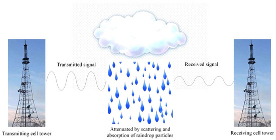
Microwave links sense rain using electromagnetic waves. Raindrops along the path absorb and scatter the signal. This causes a drop in the Received Signal Level (RSL).

We compute the Total Loss ($TL$, dB) as:

$$TL(t) = TSL(t) - RSL(t)$$

Where:

$TSL(t)$ is the Transmitted Signal Level (dBm) at time $t$.
$RSL(t)$ is the Received Signal Level (dBm) at time $t$.

Python

# Calculate Total Loss network-wide at 1-minute resolution
ds_cmls['tl'] = ds_cmls.tsl - ds_cmls.rsl

# Select the first representative CML (CML 268 has 2 fully active channels)
ds_cml = ds_cmls.sel(cml_id='268')

freq_static = ds_cml.frequency.isel(time=0) if 'time' in ds_cml.frequency.dims else ds_cml.frequency
freq_val = float(freq_static.isel(sublink_id=0))
freq_ghz = freq_val / 1000 if freq_val < 1e6 else freq_val / 1e9
print(f"Selected Link ID: {ds_cml.cml_id.values} | Path Length: {float(ds_cml.length)/1000:.2f} km | Frequency: {freq_ghz:.2f} GHz")

# Plot TSL, RSL, and TL in a stacked layout to see the raw variables for both sublinks
fig, axes = plt.subplots(3, 1, figsize=(14, 9), sharex=True)

# TSL Subplot (both sublinks)
ds_cml.tsl.isel(sublink_id=0).plot.line(x='time', ax=axes[0], color='blue', alpha=0.8, linewidth=1.5, label='Sublink 1 (Channel 1)')
ds_cml.tsl.isel(sublink_id=1).plot.line(x='time', ax=axes[0], color='orange', alpha=0.8, linewidth=1.5, label='Sublink 2 (Channel 2)')
axes[0].set_title("Transmitted Signal Level (TSL) - Constant or ATPC Adjusted", fontsize=11, fontweight='bold')
axes[0].set_ylabel("TSL (dBm)", fontweight='bold')
axes[0].legend(loc='upper right')

# RSL Subplot (both sublinks)
ds_cml.rsl.isel(sublink_id=0).plot.line(x='time', ax=axes[1], color='blue', alpha=0.8, linewidth=1.5, label='Sublink 1 (Channel 1)')
ds_cml.rsl.isel(sublink_id=1).plot.line(x='time', ax=axes[1], color='orange', alpha=0.8, linewidth=1.5, label='Sublink 2 (Channel 2)')
axes[1].set_title("Received Signal Level (RSL) - Drops during Rain", fontsize=11, fontweight='bold')
axes[1].set_ylabel("RSL (dBm)", fontweight='bold')
axes[1].legend(loc='upper right')

# TL Subplot (both sublinks)
ds_cml.tl.isel(sublink_id=0).plot.line(x='time', ax=axes[2], color='blue', alpha=0.8, linewidth=1.5, label='Sublink 1 (Channel 1)')
ds_cml.tl.isel(sublink_id=1).plot.line(x='time', ax=axes[2], color='orange', alpha=0.8, linewidth=1.5, label='Sublink 2 (Channel 2)')
axes[2].set_title("Total Loss (TL = TSL - RSL) - Increases during Rain", fontsize=11, fontweight='bold')
axes[2].set_ylabel("Total Loss (dB)", fontweight='bold')
axes[2].set_xlabel("Time (UTC)", fontweight='bold')
axes[2].legend(loc='upper right')

plt.tight_layout()
plt.show()

Section 2: Perform Processing for a CML

Now we build the core processing pipeline at 1-minute resolution. We will retrieve rain rates from raw signal attenuation on a representative path.

Step 2.1: Preprocessing & Cleaning

Signal telemetry can contain short dropouts (NaNs). We perform linear interpolation to clean these short telemetry gaps.

Python

print("NaN count in Received Signal Level before interpolation:", int(ds_cmls.rsl.isnull().sum()))

# Interpolate NaNs along the time dimension with a limit of 5 consecutive steps (5 minutes)
ds_cmls = ds_cmls.interpolate_na(dim='time', max_gap=pd.Timedelta('5min'), method='linear')
print("NaN count in Received Signal Level after interpolation:", int(ds_cmls.rsl.isnull().sum()))

# Recalculate Total Loss on the cleaned telemetry data
ds_cmls['tl'] = ds_cmls.tsl - ds_cmls.rsl
print("Total Loss (TL) successfully recalculated on cleaned dataset.")

Spotlight 1: Wet/Dry Classification

We need to detect when it is raining. This lets us separate rain-induced attenuation from clear-sky signal drift.

We calculate the Rolling Standard Deviation ($\sigma_{TL}$, dB) of the Total Loss over a symmetric 60-minute window:

$$\sigma_{TL}(t) = \text{std}\big(\{TL(t') \mid t' \in [t - 30\text{ min}, t + 30\text{ min}]\}\big)$$

Rain causes high, rapid signal fluctuations compared to dry weather. We compare two thresholding methods:

Fixed Threshold (Cite: Schleiß et al. 2010): $$\text{Wet}(t) = \sigma_{TL}(t) > 0.4\text{ dB}$$
Adaptive Threshold (Cite: Graf et al. 2020): $$\text{Threshold}_{adaptive} = 1.4 \times \text{Percentile}_{80}(\sigma_{TL})$$ This accounts for individual link hardware noise.

Python

# Helper function to highlight wet periods on plots
def highlight_wet_periods(da_wet, ax):
    # Set first and last time stamp to False to handle rolls safely
    da_wet = da_wet.copy()
    da_wet = da_wet.where(da_wet.time != da_wet.time.isel(time=0), False)
    da_wet = da_wet.where(da_wet.time != da_wet.time.isel(time=-1), False)

    wet_vals = da_wet.values.astype(bool)
    wet_start = np.roll(wet_vals, -1) & ~wet_vals
    wet_end = np.roll(wet_vals, 1) & ~wet_vals

    # Plot shaded area for each wet event using a soft transparent blue
    starts = wet_start.nonzero()[0]
    ends = wet_end.nonzero()[0]
    for idx_start, idx_end in zip(starts, ends):
        safe_end = min(idx_end, len(da_wet.time.values) - 1)
        ax.axvspan(
            da_wet.time.values[idx_start],
            da_wet.time.values[safe_end],
            color='royalblue', alpha=0.15
        )

# Select representative link
ds_cml = ds_cmls.sel(cml_id='268')

# Compute Rolling standard deviation (60-minute window) at 1-minute resolution
ds_cml['rsd'] = ds_cml.tl.rolling(time=60, center=True).std()

# Method 1: Fixed threshold
fixed_thresh = 0.4
ds_cml['wet_fixed'] = ds_cml.rsd > fixed_thresh

# Method 2: Adaptive threshold (Graf et al. 2020) - compute over the time dimension specifically
factor = 1.4
adaptive_thresh = factor * ds_cml.rsd.quantile(0.80, dim='time')
ds_cml['wet_adaptive'] = ds_cml.rsd > adaptive_thresh

# Plot both thresholds and wet classifications side-by-side
fig, axs = plt.subplots(4, 1, figsize=(14, 10), sharex=True)

# Subplot 0 & 1: Fixed Threshold
ds_cml.rsd.isel(sublink_id=0).plot.line(x='time', ax=axs[0], color='purple')
axs[0].axhline(fixed_thresh, color='k', linestyle='--', label=f'Fixed Threshold ({fixed_thresh} dB)')
axs[0].set_ylabel('RSD (dB)', fontweight='bold')
axs[0].legend(loc='upper right')
axs[0].set_title('Method 1: Fixed Threshold (Schleiß et al. 2010)', fontweight='bold')

ds_cml.tl.isel(sublink_id=0).plot.line(x='time', ax=axs[1], color='black', alpha=0.6)
highlight_wet_periods(ds_cml.wet_fixed.isel(sublink_id=0), ax=axs[1])
axs[1].set_ylabel('Total Loss (dB)', fontweight='bold')
axs[1].set_title('TL with Highlighted Fixed Wet Periods (Blue)', fontweight='bold')

# Subplot 2 & 3: Adaptive Threshold
ds_cml.rsd.isel(sublink_id=0).plot.line(x='time', ax=axs[2], color='teal')
axs[2].axhline(float(adaptive_thresh.isel(sublink_id=0)), color='k', linestyle='--',
               label=f'Adaptive Threshold ({float(adaptive_thresh.isel(sublink_id=0)):.2f} dB)')
axs[2].set_ylabel('RSD (dB)', fontweight='bold')
axs[2].legend(loc='upper right')
axs[2].set_title('Method 2: Adaptive Threshold (Graf et al. 2020)', fontweight='bold')

ds_cml.tl.isel(sublink_id=0).plot.line(x='time', ax=axs[3], color='black', alpha=0.6)
highlight_wet_periods(ds_cml.wet_adaptive.isel(sublink_id=0), ax=axs[3])
axs[3].set_ylabel('Total Loss (dB)', fontweight='bold')
axs[3].set_xlabel('Time (UTC)', fontweight='bold')
axs[3].set_title('TL with Highlighted Adaptive Wet Periods (Blue)', fontweight='bold')

plt.tight_layout()

Spotlight 2: Wet Antenna Attenuation (WAA) Models

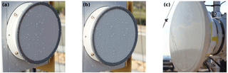
When it rains, water droplets cling to the antenna radomes. This causes additional signal loss called Wet Antenna Attenuation (WAA). WAA lingers even after the rain stops. We must subtract WAA to isolate the pure rain attenuation $A_{rain}$.

We compare three WAA retrieval models:

No WAA Correction: Directly subtract baseline ($B$) from Total Loss. This ignores radome wetting: $$A_{rain}(t) = TL(t) - B(t)$$
Time-dependent WAA (Cite: Schleiss et al. 2013): WAA increases during rain and decays exponentially during dry periods: $$WAA(t) = WAA(t-1) \cdot e^{-\Delta t / \tau}$$ Here, $\tau$ represents the radome drying time constant (e.g., 15 minutes).
Intensity-dependent WAA (Cite: Pastorek et al. 2022): WAA is modeled as an instantaneous function of the observed total attenuation $A_{obs} = TL - B$: $$WAA(t) = A_{max} \cdot \left(1 - e^{-\zeta \cdot A_{obs}(t)}\right)$$

Why the WAA models are approximating

Radome wetting is a complex physical process. It depends on wind, temperature, radome material, and evaporation.

The Schleiss et al. 2013 model tracks history using the decay constant $\tau$. The Pastorek et al. 2022 model approximates WAA using the instantaneous attenuation $A_{obs}$. Because rain intensity and radome wetness correlate during rain, this approximation works well and avoids accumulating error from historical tracking state.

Python

# Compute both baseline models:
# 1. Baseline with Fixed threshold
baseline_fixed = pycml.processing.baseline.baseline_constant(
    trsl=ds_cml.tl,
    wet=ds_cml.wet_fixed,
    n_average_last_dry=30
)
ds_cml['baseline_fixed'] = baseline_fixed

# 2. Baseline with Adaptive threshold
baseline_adaptive = pycml.processing.baseline.baseline_constant(
    trsl=ds_cml.tl,
    wet=ds_cml.wet_adaptive,
    n_average_last_dry=30
)
ds_cml['baseline_adaptive'] = baseline_adaptive
ds_cml['baseline'] = baseline_adaptive  # Shortcut for plotting

# Model A: Time-dependent WAA (Schleiss 2013) using Adaptive wet/dry classification
# Run waa_schleiss_2013 channel-by-channel to match the 1D input requirement of the wrapper
waa_s_list = []

# Sublink 1 (Channel 1) calculation
waa_ch1 = pycml.processing.wet_antenna.waa_schleiss_2013(
    rsl=ds_cml.tl.isel(sublink_id=0).values,
    baseline=ds_cml.baseline_adaptive.isel(sublink_id=0).values,
    wet=ds_cml.wet_adaptive.isel(sublink_id=0).values,
    waa_max=2.0,
    delta_t=1.0,
    tau=15.0
)
waa_s_list.append(waa_ch1)

# Sublink 2 (Channel 2) calculation
waa_ch2 = pycml.processing.wet_antenna.waa_schleiss_2013(
    rsl=ds_cml.tl.isel(sublink_id=1).values,
    baseline=ds_cml.baseline_adaptive.isel(sublink_id=1).values,
    wet=ds_cml.wet_adaptive.isel(sublink_id=1).values,
    waa_max=2.0,
    delta_t=1.0,
    tau=15.0
)
waa_s_list.append(waa_ch2)

ds_cml['waa_schleiss'] = (('sublink_id', 'time'), np.stack(waa_s_list))

# Model B: Intensity-dependent WAA (Pastorek 2021) using Adaptive baseline
A_obs_adaptive = ds_cml.tl - ds_cml.baseline_adaptive
A_obs_adaptive = A_obs_adaptive.where(A_obs_adaptive >= 0, 0)
freq_static = ds_cml.frequency.isel(time=0) if 'time' in ds_cml.frequency.dims else ds_cml.frequency
freq_hz = freq_static * 1e6 if float(freq_static.isel(sublink_id=0)) < 1e6 else freq_static

waa_pastorek = pycml.processing.wet_antenna.waa_pastorek_2021_from_A_obs(
    A_obs=A_obs_adaptive,
    f_Hz=freq_hz,
    pol=ds_cml.polarization.data,
    L_km=ds_cml.length / 1000,
    A_max=2.0,
    zeta=0.7,
    d=0.15
)
ds_cml['waa_pastorek'] = waa_pastorek

# Calculate pure rain-induced attenuation (A) for each configuration
ds_cml['A_fixed_no_waa'] = (ds_cml.tl - ds_cml.baseline_fixed).where(lambda x: x > 0, 0)
ds_cml['A_adaptive_no_waa'] = (ds_cml.tl - ds_cml.baseline_adaptive).where(lambda x: x > 0, 0)
ds_cml['A_adaptive_pastorek'] = (ds_cml.tl - ds_cml.baseline_adaptive - ds_cml.waa_pastorek).where(lambda x: x > 0, 0)
ds_cml['A_adaptive_schleiss'] = (ds_cml.tl - ds_cml.baseline_adaptive - ds_cml.waa_schleiss).where(lambda x: x > 0, 0)

# Keep standard variables for plotting
ds_cml['A_schleiss'] = ds_cml.A_adaptive_schleiss
ds_cml['A_pastorek'] = ds_cml.A_adaptive_pastorek
ds_cml['A_no_waa'] = ds_cml.A_adaptive_no_waa

# Invert attenuation to rain rate (R) using ITU-R P.838 power law
f_ghz = freq_static / 1000 if float(freq_static.isel(sublink_id=0)) > 1000 else freq_static
for m in ['fixed_no_waa', 'adaptive_no_waa', 'adaptive_pastorek', 'adaptive_schleiss']:
    ds_cml[f'R_{m}'] = pycml.processing.k_R_relation.calc_R_from_A(
        A=ds_cml[f'A_{m}'],
        L_km=float(ds_cml.length)/1000,
        f_GHz=f_ghz,
        pol=ds_cml.polarization
)

# Keep standard variables for plotting
ds_cml['R_schleiss'] = ds_cml.R_adaptive_schleiss
ds_cml['R_pastorek'] = ds_cml.R_adaptive_pastorek
ds_cml['R_no_waa'] = ds_cml.R_adaptive_no_waa

# Assign default retrieved rain rate for downstream validation to 'R_adaptive_pastorek'
ds_cml['R'] = ds_cml.R_adaptive_pastorek
print("WAA comparative calculations completed successfully!")

Let's zoom into a major rain event and compare the baseline, pure rain attenuation, and inverted rain rate across all three WAA configurations, alongside the collocated weather radar.

Python

# Zoom in on a major rain event at the start of the selected month
if selected_month == "2021-01":
    t_start_zoom, t_end_zoom = "2021-01-01 00:00:00", "2021-01-03 23:59:00"
else:
    t_start_zoom, t_end_zoom = "2021-11-01 00:00:00", "2021-11-03 23:59:00"

ds_cml_zoom = ds_cml.sel(time=slice(t_start_zoom, t_end_zoom))

fig, axs = plt.subplots(3, 1, figsize=(14, 11), sharex=True)

# Subplot 0: Total Loss and Baselines
ds_cml_zoom.tl.isel(sublink_id=0).plot.line(x='time', ax=axs[0], color='black', alpha=0.4, label='Total Loss (TL)', linewidth=1.5)
ds_cml_zoom.baseline.isel(sublink_id=0).plot.line(x='time', ax=axs[0], color='red', linestyle='--', label='Baseline without WAA (Constant)', linewidth=2.0)
(ds_cml_zoom.baseline + ds_cml_zoom.waa_schleiss).isel(sublink_id=0).plot.line(x='time', ax=axs[0], color='purple', linestyle=':', label='Baseline + WAA (Schleiss 2013 Decay)', linewidth=2.0)
(ds_cml_zoom.baseline + ds_cml_zoom.waa_pastorek).isel(sublink_id=0).plot.line(x='time', ax=axs[0], color='blue', linestyle='-.', label='Baseline + WAA (Pastorek 2021 Instantaneous)', linewidth=2.0)
axs[0].set_title("Total Loss & Baseline Comparisons", fontsize=12, fontweight='bold')
axs[0].set_ylabel("Signal Level (dB)", fontweight='bold')
axs[0].legend(frameon=True, loc='upper right')

# Subplot 1: Pure Rain Attenuation
ds_cml_zoom.A_pastorek.isel(sublink_id=0).plot.line(x='time', ax=axs[1], color='blue', label='Rain Attenuation (Pastorek 2021)', linewidth=2.0)
ds_cml_zoom.A_schleiss.isel(sublink_id=0).plot.line(x='time', ax=axs[1], color='purple', linestyle='--', label='Rain Attenuation (Schleiss 2013)', linewidth=1.8)
ds_cml_zoom.A_no_waa.isel(sublink_id=0).plot.line(x='time', ax=axs[1], color='gray', linestyle=':', label='Rain Attenuation (No WAA)', linewidth=1.5)
axs[1].set_title("Pure Rain Attenuation Comparison (A_rain)", fontsize=12, fontweight='bold')
axs[1].set_ylabel("Attenuation (dB)", fontweight='bold')
axs[1].legend(frameon=True, loc='upper right')

# Subplot 2: Rain Rate Inversion vs Radar
ds_cml_zoom.R_pastorek.isel(sublink_id=0).plot.line(x='time', ax=axs[2], color='blue', label='CML Rain (Pastorek 2021)', linewidth=2.0)
ds_cml_zoom.R_schleiss.isel(sublink_id=0).plot.line(x='time', ax=axs[2], color='purple', linestyle='--', label='CML Rain (Schleiss 2013)', linewidth=1.8)
ds_cml_zoom.R_no_waa.isel(sublink_id=0).plot.line(x='time', ax=axs[2], color='gray', linestyle=':', label='CML Rain (No WAA)', linewidth=1.5)

# Extract collocated radar time series
radar_zoom = cmls_R_radar.sel(cml_id=ds_cml.cml_id).sel(time=slice(t_start_zoom, t_end_zoom))
radar_zoom.plot.line(x='time', ax=axs[2], color='black', label='Radar along CML', linewidth=1.5)

axs[2].set_title("Retrieved Rain Rate Comparison vs. Weather Radar", fontsize=12, fontweight='bold')
axs[2].set_ylabel("Rain Rate (mm/h)", fontweight='bold')
axs[2].set_xlabel("Time (UTC)", fontweight='bold')
axs[2].legend(frameon=True, loc='upper right')

plt.tight_layout()
plt.show()

Section 3: Validation and Comparison

We validate our CML-derived rain rates against rain gauges and weather radar.

Native 15-Minute Resampling

Physical rain gauges measure accumulated rainfall depth ($d_{15m}$, mm) over 15-minute intervals. To compare CMLs and gauges fairly, we resample CML estimates to the same 15-minute grid:

CML 15-Min Mean Rain Rate ($R_{CML, 15m}$, mm/h): We calculate the average CML rain rate over each 15-minute window.
Gauge 15-Min equivalent Intensity ($R_{gauge, 15m}$, mm/h): We multiply the 15-minute gauge rain depth by 4 to get its hourly intensity equivalent: $$R_{gauge, 15m} = d_{15m} \times 4.0$$

Step 3.1: Close-Gauge Time Series Validation

We plot the resampled 15-minute CML rain rate against the nearest rain gauge.

Python

# Isolate closest gauge data for our selected CML path
nearest_gauge_id = closest_neighbors.sel(cml_id=ds_cml.cml_id).neighbor_id.values[0]
ds_closest_gauge = ds_gauges.sel(id=nearest_gauge_id)
distance_m = closest_neighbors.sel(cml_id=ds_cml.cml_id).distance.values[0]
print(f"Closest Gauge ID: {nearest_gauge_id} | Distance: {distance_m:.1f} meters")

# Resample CML versions and Gauge to 15-minute intervals matching the native sampling
cml_fixed_15m = ds_cml.R_fixed_no_waa.isel(sublink_id=0).resample(time='15min').mean()
cml_adaptive_15m = ds_cml.R_adaptive_no_waa.isel(sublink_id=0).resample(time='15min').mean()
cml_pastorek_15m = ds_cml.R_adaptive_pastorek.isel(sublink_id=0).resample(time='15min').mean()
gauge_15m = ds_closest_gauge.rainfall_amount.resample(time='15min').sum() * 4.0

# Plot validation comparison in subplots
fig, axs = plt.subplots(3, 1, figsize=(14, 12), sharex=True)

# Subplot 0: Fixed 0.4 dB Thresh, No WAA vs Pluviometer
cml_fixed_15m.plot.line(
    x='time', ax=axs[0], color='gray', linestyle=':', label='CML (0.4dB Thresh, No WAA)', linewidth=1.5
)
gauge_15m.plot.line(
    x='time', ax=axs[0], color='black', label=f'ARPAE Pluviometer [{nearest_gauge_id}]', linestyle='--', linewidth=1.8
)
axs[0].set_title("Configuration 1: Fixed Threshold (0.4 dB) vs. Pluviometer", fontsize=11, fontweight='bold')
axs[0].set_ylabel("Intensity (mm/h)", fontweight='bold')
axs[0].legend(frameon=True, loc='upper right')

# Subplot 1: Adaptive Thresh, No WAA vs Pluviometer
cml_adaptive_15m.plot.line(
    x='time', ax=axs[1], color='teal', linestyle='-.', label='CML (Adaptive Thresh, No WAA)', linewidth=1.8
)
gauge_15m.plot.line(
    x='time', ax=axs[1], color='black', label=f'ARPAE Pluviometer [{nearest_gauge_id}]', linestyle='--', linewidth=1.8
)
axs[1].set_title("Configuration 2: Adaptive Threshold vs. Pluviometer", fontsize=11, fontweight='bold')
axs[1].set_ylabel("Intensity (mm/h)", fontweight='bold')
axs[1].legend(frameon=True, loc='upper right')

# Subplot 2: Adaptive Thresh + Pastorek WAA vs Pluviometer
cml_pastorek_15m.plot.line(
    x='time', ax=axs[2], color='royalblue', label='CML (Adaptive Thresh + Pastorek WAA)', linewidth=2.2
)
gauge_15m.plot.line(
    x='time', ax=axs[2], color='black', label=f'ARPAE Pluviometer [{nearest_gauge_id}]', linestyle='--', linewidth=1.8
)
axs[2].set_title("Configuration 3: Adaptive Threshold + Pastorek 2021 WAA vs. Pluviometer", fontsize=11, fontweight='bold')
axs[2].set_ylabel("Intensity (mm/h)", fontweight='bold')
axs[2].set_xlabel("Time (UTC)", fontweight='bold')
axs[2].legend(frameon=True, loc='upper right')

plt.tight_layout()
plt.show()

Step 3.2: Triple-Sensor Correlation Analysis

We calculate the Pearson correlation matrix. This compares CML estimates, radar grid pixels, and physical rain gauge records.

Python

# Resample CML versions, Radar, and Gauge to 15-minute intervals
cml_fixed_15m = ds_cml.R_fixed_no_waa.isel(sublink_id=0).resample(time='15min').mean()
cml_adaptive_15m = ds_cml.R_adaptive_no_waa.isel(sublink_id=0).resample(time='15min').mean()
cml_pastorek_15m = ds_cml.R_adaptive_pastorek.isel(sublink_id=0).resample(time='15min').mean()

radar_15m = cmls_R_radar.sel(cml_id=ds_cml.cml_id).resample(time='15min').mean()
gauge_15m = ds_closest_gauge.rainfall_amount.resample(time='15min').sum() * 4.0

# Align timestamps
common_time = np.intersect1d(
    np.intersect1d(
        np.intersect1d(cml_fixed_15m.time.values, cml_adaptive_15m.time.values),
        cml_pastorek_15m.time.values
    ),
    np.intersect1d(radar_15m.time.values, gauge_15m.time.values)
)

# Construct DataFrame
df_corr = pd.DataFrame({
    'CML (0.4dB Thresh)': cml_fixed_15m.sel(time=common_time).values,
    'CML (Adaptive Thresh)': cml_adaptive_15m.sel(time=common_time).values,
    'CML (Adaptive+Pastorek WAA)': cml_pastorek_15m.sel(time=common_time).values,
    'Radar': radar_15m.sel(time=common_time).values,
    'Rain Gauge': gauge_15m.sel(time=common_time).values
})

# Compute Pearson correlation matrix
corr_matrix = df_corr.corr()
print("Pearson Correlation Matrix (15-Minute Resolution):")
print(corr_matrix)

# Plot correlation matrix heatmap
fig, ax = plt.subplots(figsize=(8, 7))
im = ax.imshow(corr_matrix, cmap='coolwarm', vmin=-1, vmax=1)

# Add text annotations for correlation values
for i in range(len(corr_matrix.columns)):
    for j in range(len(corr_matrix.columns)):
        ax.text(j, i, f"{corr_matrix.iloc[i, j]:.3f}", ha='center', va='center',
                color='white' if abs(corr_matrix.iloc[i, j]) > 0.5 else 'black',
                fontweight='bold', fontsize=12)

ax.set_xticks(np.arange(len(corr_matrix.columns)))
ax.set_yticks(np.arange(len(corr_matrix.columns)))
ax.set_xticklabels(corr_matrix.columns, fontweight='bold', fontsize=10, rotation=15)
ax.set_yticklabels(corr_matrix.columns, fontweight='bold', fontsize=10)
ax.set_title("Triple-Sensor Rainfall Correlation Showdown", fontsize=13, fontweight='bold')

# Add colorbar
cbar = plt.colorbar(im, ax=ax, shrink=0.8)
cbar.set_label("Pearson Correlation Coefficient", fontweight='bold')

plt.tight_layout()
plt.show()

Step 3.3: Network-Wide Processing

To evaluate the entire network, we run our processing pipeline across all filtered links. We wrap the 5-step retrieval pipeline inside a reusable helper function process_cml_empirical(ds_link). Then, we process all links using a clean list comprehension.

Python

# Create a clean helper function to process any link
def process_cml_empirical(ds_link):
    # 1. Wet/Dry (Adaptive Threshold)
    rsd = ds_link.tl.rolling(time=60, center=True).std()
    wet = rsd > (1.4 * rsd.quantile(0.80, dim='time'))

    # 2. Baseline
    baseline = pycml.processing.baseline.baseline_constant(ds_link.tl, wet, 30)
    A_obs = (ds_link.tl - baseline).clip(min=0)

    # 3. WAA (Pastorek 2021)
    f_hz = (ds_link.frequency * 1e6).isel(time=0) if float(ds_link.frequency.isel(time=0, sublink_id=0)) < 1e6 else ds_link.frequency.isel(time=0)
    waa = pycml.processing.wet_antenna.waa_pastorek_2021_from_A_obs(
        A_obs,
        f_hz,
        ds_link.polarization.data,
        float(ds_link.length)/1000,
        2.0,
        0.7,
        0.15
    )

    # 4. Pure Rain
    A_rain = (ds_link.tl - baseline - waa).clip(min=0)

    # 5. Inversion
    return pycml.processing.k_R_relation.calc_R_from_A(
        A_rain,
        float(ds_link.length)/1000,
        f_hz/1e9,
        ds_link.polarization
    )

# Process all CML paths network-wide using the clean helper function
print("Processing all CML paths network-wide...")
R_list = [process_cml_empirical(ds_cmls.sel(cml_id=cid)) for cid in ds_cmls.cml_id.values]

# Merge back to the master dataset
ds_cmls['R'] = xr.concat(R_list, dim='cml_id')

# Resample CML to 15-minute mean and match dimensions with Radar
cml_R_15m = ds_cmls.R.isel(sublink_id=0).resample(time='15min').mean()
cml_R_15m = cml_R_15m.transpose('time', 'cml_id')

# Align timestamps
common_time = np.intersect1d(cmls_R_radar.time.values, cml_R_15m.time.values)
ref = cmls_R_radar.sel(time=common_time).values.flatten()
est = cml_R_15m.sel(time=common_time).values.flatten()

# Calculate validation metrics
metrics = plg.validation.calculate_rainfall_metrics(ref, est, ref_thresh=0.1, est_thresh=0.1)
plg.validation.print_metrics_table(metrics)

# Generate hexbin scatter plot
fig, ax = plt.subplots(figsize=(8, 7))
plg.validation.plot_hexbin(ref, est, ref_thresh=0.1, est_thresh=0.1, gridsize=45, ax=ax)
ax.set_title("Precipitation Showdown: CML vs. Radar Colocation (Adaptive Thresh + WAA)", fontsize=13, fontweight='bold')
ax.set_xlabel("Radar Rainfall Reference (mm/h)", fontweight='bold')
ax.set_ylabel("CML Estimated Rainfall (mm/h)", fontweight='bold')
plt.tight_layout()
plt.show()

Section 4: Spotlight 3 – Nearby-Link Consensus & The Temporal Gap (RAINLINK)

Here, we explore how spatial density is used to retrieve rain rates from legacy networks. These legacy networks only report aggregated 15-minute min-max data.

The "Nearby-Link" Consensus Algorithm

RAINLINK is developed for legacy Network Monitoring Systems (NMS) (Cite: Overeem et al. 2016). It establishes wet/dry states by demanding spatial agreement between neighboring links:

Min-Max Telemetry: NMS systems record the 15-minute minimum and maximum Received Signal Levels (pmin, pmax).
Spatial Consensus: A link is classified as Wet if a minimum number of neighboring links within a radius $r$ (e.g., 15 km) also experience a signal drop. This consensus step filters out local hardware glitches.

The Temporal Aggregation Gap

Aggregating high-resolution 1-minute telemetry into 15-minute bins flattens peak rain intensities. We compare the 15-minute RAINLINK retrieval against our 1-minute RSD retrieval to visually prove this peak flattening (Cite: van der Valk et al. 2024).

Spatial Consensus Density Notice

In this spotlight section, we switch our target link to CML ID 364 (located in the dense Bologna city cluster). Because link 268 is situated in a sparse network area, it does not have the minimum density of neighboring links (at least 3 links within a 15 km radius) required by RAINLINK's spatial consensus filter, resulting in empty (NaN) outputs. Link 364 resides in a dense neighborhood, making it the ideal candidate to demonstrate the temporal gap.

Python

import pycomlink.processing.wet_dry.nearby_wetdry as nearby_wetdry
import pycomlink.processing.nearby_rain_retrival as nearby_rain

print("Simulating legacy 15-minute monitoring network (NMS min-max)...")
# Open the full NetCDF dataset to get all 18 CML paths (including short ones) for spatial density
ds_cmls_full = xr.open_dataset("data/cml/po_valley_cmls.nc").sel(time=selected_month).load()
ds_cmls_full['tl'] = ds_cmls_full.tsl - ds_cmls_full.rsl
ds_cmls_full = ds_cmls_full.interpolate_na(dim='time', max_gap=pd.Timedelta('5min'), method='linear')
ds_cmls_full['tl'] = ds_cmls_full.tsl - ds_cmls_full.rsl

# Compute 15-minute min and max signal drops (RSL - TSL)
rstl = ds_cmls_full.rsl - ds_cmls_full.tsl
pmin = rstl.resample(time="15min").min()
pmax = rstl.resample(time="15min").max()
pmin['length'] = pmin.length / 1e3  # Convert meters to km for RAINLINK

# Calculate geographic distances between endpoints for the consensus neighborhood
print("Calculating distances between CML endpoints...")
ds_dist = nearby_wetdry.calc_distance_between_cml_endpoints(
    cml_ids=ds_cmls_full.cml_id.values,
    site_a_latitude=ds_cmls_full.site_0_lat.values,
    site_a_longitude=ds_cmls_full.site_0_lon.values,
    site_b_latitude=ds_cmls_full.site_1_lat.values,
    site_b_longitude=ds_cmls_full.site_1_lon.values,
)

# Run nearby-link wet/dry consensus
print("Running nearby-link spatial consensus wet/dry classification...")
wet, F = nearby_wetdry.nearby_wetdry(
    pmin=pmin,
    ds_dist=ds_dist,
    radius=15,
    thresh_median_P=-1.4,
    thresh_median_PL=-0.7,
    min_links=3,
    interval=15,
    timeperiod=24,
)

# Estimate reference level and correct min-max signals
print("Determining reference baseline and correcting signals...")
pref = nearby_rain.nearby_determine_reference_level(pmin, pmax, wet, n_average_dry=96, min_periods=1)
p_c_min, p_c_max = nearby_rain.nearby_correct_received_signals(pmin, pmax, wet, pref)

# Extract frequencies and convert to GHz
freq_static_all = ds_cmls_full.frequency.isel(time=0) if 'time' in ds_cmls_full.frequency.dims else ds_cmls_full.frequency
freq_val = float(freq_static_all.isel(cml_id=0, sublink_id=0).values)
f_ghz_all = freq_static_all / 1e3 if freq_val > 1000 else freq_static_all

# Run RAINLINK nearby rainfall retrieval (using positional parameters to avoid wrapper keyword bugs)
print("Retrieving rain rates using RAINLINK consensus...")
R_nearby = nearby_rain.nearby_rainfall_retrival(
    pref,
    p_c_min,
    p_c_max,
    F,
    pmin.length,
    f_GHz=f_ghz_all,
    pol=pmin.polarization,
    waa_max=2.3,
    alpha=0.33,
    F_value_threshold=-32.5,
)
print("RAINLINK nearby retrieval completed successfully!")
ds_cmls_full.close()

Python

# Extract 1-minute RSD-based rain rate for link '364' (processed network-wide previously)
R_rsd_cml = ds_cmls.sel(cml_id="364").R.isel(sublink_id=0)

# Extract 15-minute RAINLINK consensus rain rate for link '364'
R_nearby_cml = R_nearby.sel(cml_id="364").isel(sublink_id=0)

# Define storm zoom window
if selected_month == "2021-01":
    t_start_zoom, t_end_zoom = "2021-01-01 00:00:00", "2021-01-03 23:59:00"
else:
    t_start_zoom, t_end_zoom = "2021-11-01 00:00:00", "2021-11-03 23:59:00"

# Slice both time series
R_rsd_zoom = R_rsd_cml.sel(time=slice(t_start_zoom, t_end_zoom))
R_nearby_zoom = R_nearby_cml.sel(time=slice(t_start_zoom, t_end_zoom))

# Plot both to demonstrate peak flattening
fig, ax = plt.subplots(figsize=(14, 6))

R_rsd_zoom.plot.line(
    ax=ax, color='crimson', linewidth=2.0, label='1-Minute RSD (Pastorek WAA)'
)
R_nearby_zoom.plot.line(
    ax=ax, color='royalblue', linewidth=2.5, linestyle='--', marker='o', markersize=4,
    label='15-Minute RAINLINK (Nearby Consensus)'
)

# Print peak values to show mathematically
peak_rsd = float(R_rsd_zoom.max(skipna=True))
peak_nearby = float(R_nearby_zoom.max(skipna=True))
print(f"Convective Storm Peak Intensity Comparison:")
print(f" * 1-Minute RSD Peak: {peak_rsd:.2f} mm/h")
print(f" * 15-Minute RAINLINK Peak: {peak_nearby:.2f} mm/h")
print(f" * Peak Reduction: {((peak_rsd - peak_nearby) / peak_rsd * 100):.1f}%")

ax.set_title("The Temporal Resolution Gap: 1-Min RSD vs. 15-Min RAINLINK Consensus (Link 364)",
             fontsize=13, fontweight='bold')
ax.set_ylabel("Rainfall Intensity (mm/h)", fontweight='bold')
ax.set_xlabel("Time (UTC)", fontweight='bold')
ax.legend(frameon=True, fontsize=11)
plt.tight_layout()
plt.show()

Session Conclusion & The "Phantom Drizzle" Problem

Let's review the insights from our validation plots, hexbin correlation, and the temporal resolution gap. We can identify three key performance challenges in standard empirical CML processing:

1. Overestimation Bias (Fog and Non-Rain Events)

The Problem: The network-wide validation shows high scatter when rain gauges read zero.
The Cause: Heavy radiation fog in the Po Valley attenuates high-frequency signals. Our simple rolling standard deviation classifies this fog as wet weather.

2. Static Wet Antenna Attenuation (WAA) Limits

The Problem: WAA models like Pastorek and Schleiss rely on static parameters ($A_{max}$, $\tau$).
The Cause: The evaporation of water off the radome depends dynamically on wind speed and temperature. Static models cannot capture these changes.

3. The Temporal Resolution Gap (Peak Flattening)

The Problem: 15-minute NMS min-max telemetry (used in RAINLINK) significantly underestimates peak rain rates.
The Cause: Aggregating signal fluctuations to 15-minute blocks mathematically averages out the intense cores of sudden convective storms.

The Path Forward: Atmospheric Thermodynamics (Advanced Session)

To solve these challenges, we must move beyond empirical signal statistics. In our next advanced session, we will introduce physical modeling:

Dynamic Baseline Tracking: We will use a 1D Kalman Filter to estimate dry-weather signal levels dynamically.
Physical Antenna Evaporation: We will integrate downscaled ERA5 weather data (temperature, wind, and relative humidity) and apply the Dalton Mass Transfer Equation to model antenna radome drying in real-time.

Key Takeaway

This physical approach eliminates fog-induced overestimation and dynamically tracks antenna drying, paving the way for next-generation opportunistic rainfall sensing!

References

Covi, F., et al. (2024). OpenRainER: An open commercial microwave link rainfall testbed in the Po Valley, Italy. Earth System Science Data (Discussions). https://doi.org/10.5194/essd-2026-160
Uijlenhoet, R., et al. (2018). Opportunistic remote sensing of rainfall using microwave links from cellular communication networks. WIREs Water, 5(4), e1289. https://doi.org/10.1002/wat2.1289
Schleiß, M., & Berne, A. (2010). Identification of dry and rainy periods using telecommunication microwave links. IEEE Geoscience and Remote Sensing Letters, 7(3), 611–615. https://doi.org/10.1109/LGRS.2010.2043052
Graf, M., et al. (2020). Rainfall estimation from a German-wide commercial microwave link network: optimized processing and validation for 1 min data. Hydrology and Earth System Sciences, 24(6), 2931–2950. https://doi.org/10.5194/hess-24-2931-2020
Schleiss, M., Rieckermann, J., & Berne, A. (2013). Quantification and modeling of wet-antenna attenuation for commercial microwave links. IEEE Geoscience and Remote Sensing Letters, 10(5), 1195–1199. https://doi.org/10.1109/LGRS.2012.2236074
Pastorek, J., et al. (2022). Wet antenna attenuation correction for microwave links using an instantaneous relation with rain-induced attenuation. IEEE Transactions on Geoscience and Remote Sensing, 60, 1–12. https://doi.org/10.1109/TGRS.2021.3110004
Overeem, A., Leijnse, H., & Uijlenhoet, R. (2016). Retrieval algorithm for rainfall mapping from microwave links in a cellular communication network. Atmospheric Measurement Techniques, 9(5), 2425–2444. https://doi.org/10.5194/amt-9-2425-2016
van der Valk, R., et al. (2024). On the temporal sampling of commercial microwave link rainfall retrieval. Atmospheric Measurement Techniques, 17(9), 2811–2827. https://doi.org/10.5194/amt-17-2811-2024

Samuel Mbugua

Table of Contents

Table of Contents

Introduction to CML Data Processing: The Po Valley (OpenRainER)

Introduction

Learning Objectives

Environment & Dependency Setup

Step 1: Library Imports

Section 1: Load and Explore CML Data

Step 1.1: Loading the Dataset

Step 1.2: Standardize Coordinates and Spatial Projection

Step 1.3: Geometric Filtering

Step 1.4: Radar Alignment

Step 1.5: Spatial Network Topography

Step 1.6: Signal Exploration (TSL, RSL, TL)

Section 2: Perform Processing for a CML

Step 2.1: Preprocessing & Cleaning

Spotlight 1: Wet/Dry Classification

Spotlight 2: Wet Antenna Attenuation (WAA) Models

Section 3: Validation and Comparison

Native 15-Minute Resampling

Step 3.1: Close-Gauge Time Series Validation

Step 3.2: Triple-Sensor Correlation Analysis

Step 3.3: Network-Wide Processing

Section 4: Spotlight 3 – Nearby-Link Consensus & The Temporal Gap (RAINLINK)

The "Nearby-Link" Consensus Algorithm

The Temporal Aggregation Gap

Session Conclusion & The "Phantom Drizzle" Problem

1. Overestimation Bias (Fog and Non-Rain Events)

2. Static Wet Antenna Attenuation (WAA) Limits

3. The Temporal Resolution Gap (Peak Flattening)

The Path Forward: Atmospheric Thermodynamics (Advanced Session)

References

Samuel Mbugua

Table of Contents

Table of Contents

Introduction

Learning Objectives

Environment & Dependency Setup

Step 1: Library Imports

Section 1: Load and Explore CML Data

Step 1.1: Loading the Dataset

Step 1.2: Standardize Coordinates and Spatial Projection

Step 1.3: Geometric Filtering

Step 1.4: Radar Alignment

Step 1.5: Spatial Network Topography

Step 1.6: Signal Exploration (TSL, RSL, TL)

Section 2: Perform Processing for a CML

Step 2.1: Preprocessing & Cleaning

Spotlight 1: Wet/Dry Classification

Spotlight 2: Wet Antenna Attenuation (WAA) Models

Section 3: Validation and Comparison

Native 15-Minute Resampling

Step 3.1: Close-Gauge Time Series Validation

Step 3.2: Triple-Sensor Correlation Analysis

Step 3.3: Network-Wide Processing

Section 4: Spotlight 3 – Nearby-Link Consensus & The Temporal Gap (RAINLINK)

The "Nearby-Link" Consensus Algorithm

The Temporal Aggregation Gap

Session Conclusion & The "Phantom Drizzle" Problem

1. Overestimation Bias (Fog and Non-Rain Events)

2. Static Wet Antenna Attenuation (WAA) Limits

3. The Temporal Resolution Gap (Peak Flattening)

The Path Forward: Atmospheric Thermodynamics (Advanced Session)

References

Related Tutorials

Graph Neural Networks for Hydrological Spatial Imputation

Introduction to NLP