Introduction to Kernel Methods

Get the complete Introduction_to_Kernel_Methods.ipynb and follow along at your own pace.

Download (.ipynb)

How to follow this tutorial

Why Do We Need Kernel Methods?

Imagine you are building a machine learning model to distinguish between apples and oranges using only two features:

• Weight
• Color intensity

You plot the data, and the classes can be separated by a straight line.

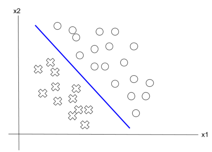
Real-world data is rarely neat, parallel lines. When data features form concentric rings, or complex structures in their native input space $\mathbb{R}^d$, a flat hyperplane is becomes unreliable in separating them.

Nonlinear Separation:

• Classes overlap and require curved decision boundaries.

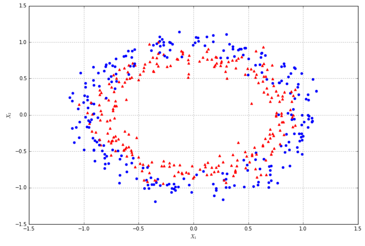
How can we classify data that is not linearly separable?

Kernel Methods

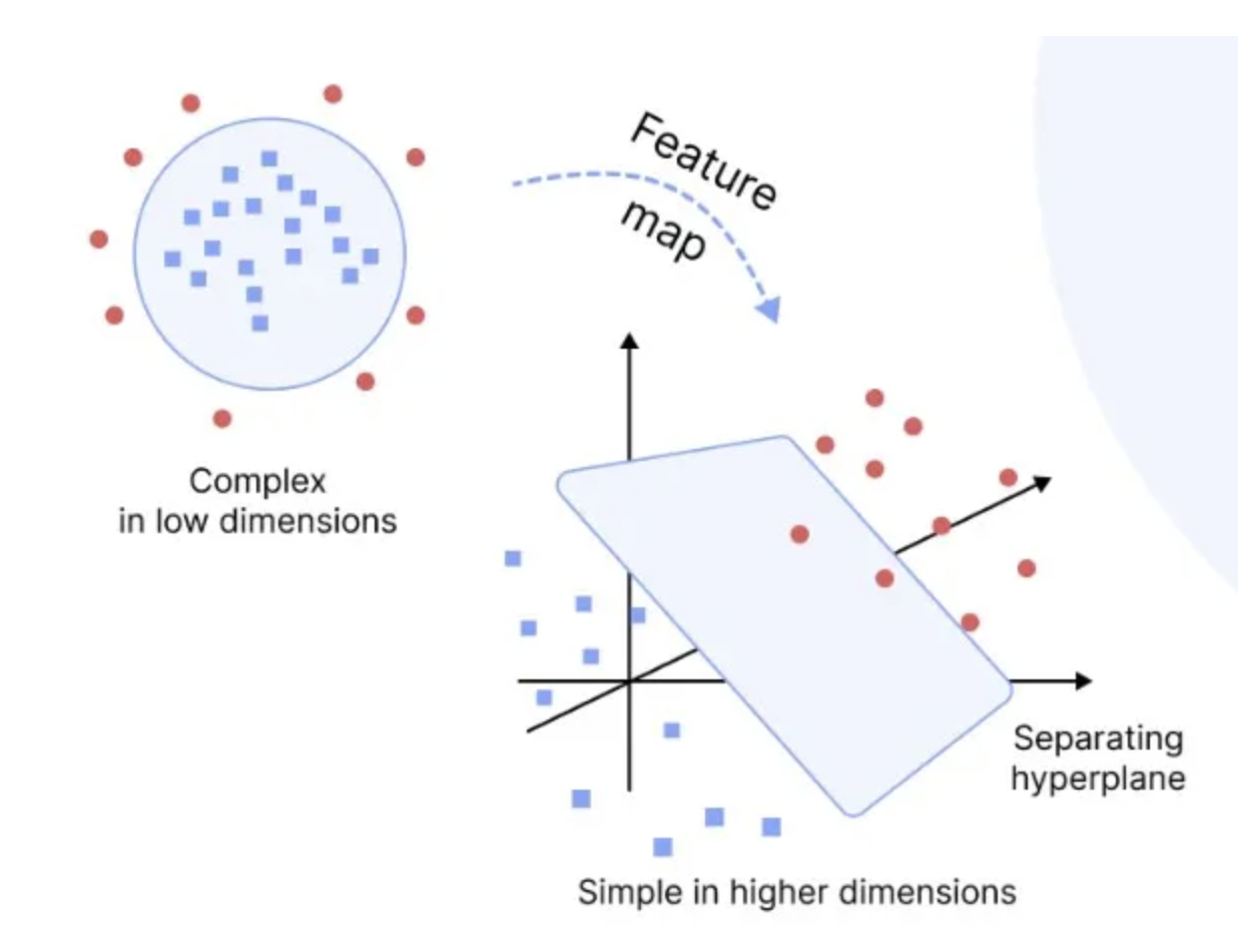
Kernel methods are a class of machine learning techniques that enable algorithms to model nonlinear relationships by implicitly mapping data into high-dimensional feature spaces.

The Feature Map ($\Phi$)

We define an explicit transformation function $\Phi: X \to H$ that takes our input vectors from our low-dimensional space $X$ and projects them into a higher-dimensional feature space $H$.

The Mathematical Transformation

Consider a 2D input vector $\mathbf{x} = [x_1, x_2]^T$. We can explicitly lift it into a 3D quadratic space using the following mapping:

Training a simple, linear classifier on these new 3D coordinates yields a perfect linear split in 3D, which projects back down as a perfectly curved quadratic circle in our original 2D space.

The Bottleneck — Dimensionality Explosion

When you map a vector of dimensionality $d$ into a polynomial space of degree $p$, the number of new feature coordinates scales combinatorially according to the binomial coefficient:

Suppose your original data has just $d = 100$ features (e.g., a tiny patch of pixels or text tokens):

• Degree $p = 2$: Your data expands to $5,151$ dimensions. This is highly manageable.
• Degree $p = 5$: Your space explodes to $96,560,646$ dimensions!

Explicitly calculating, storing, and running gradient descent over a 96-million-dimensional vector for thousands of samples will immediately exhaust your hardware's memory and cause your compute pipeline to crash.

Kernel Trick

The Hidden Structural Loophole

If you look closely at the underlying optimization mathematics for linear classifiers (like the dual formulation of an SVM), you will find something fascinating: the data vectors only ever interact via an inner dot product:

Kernel Definition

A Kernel function $K(\mathbf{x}_i, \mathbf{x}_j)$ is a mathematical shortcut. It calculates the exact dot product of vectors in that high-dimensional feature space $H$ directly using the coordinates in the original low-dimensional space, without ever calculating the explicit coordinate transformation $\Phi(\cdot)$.

Let's mathematically prove that a simple kernel function yields the exact same numerical result as an explicit high-dimensional transformation.

• Given: Two 2D vectors, $\mathbf{x} = [x_1, x_2]^T$ and $\mathbf{z} = [z_1, z_2]^T$.
• Kernel Choice: We choose a Polynomial Kernel of degree 2: $K(\mathbf{x}, \mathbf{z}) = (\mathbf{x}^T\mathbf{z})^2$.

Step 1: Compute the Kernel Shortcut directly in the original 2D space

Step 2: Evaluate the Explicit Dot Product in the 3D feature space

Using our mapping function, $\Phi(\mathbf{x}) = [x_1^2, \sqrt{2}x_1x_2, x_2^2]^T$ and $\Phi(\mathbf{z}) = [z_1^2, \sqrt{2}z_1z_2, z_2^2]^T$:

Note

Step 1 and Step 2 yield the exact same algebraic expression.

The Kernel function allowed us to completely skip calculating the square roots ($\sqrt{2}$) and storing the 3D vectors entirely, computing the high-dimensional similarity instantly.

Common Kernel Functions

1. Linear Kernel

• $K(x,z)=x^Tz$

2. Polynomial Kernel

• $K(x,z)=(x^Tz+c)^d$

3. Gaussian (RBF) Kernel

• $K(x,z) = e^{-\gamma ||x-z||^2}$

4. Sigmoid Kernel

• $K(x,z)=\tanh(\alpha x^Tz+c)$

Applications of Kernel Methods

Computer Vision

• Face Recognition: In face recognition systems, high-dimensional variations caused by lighting changes, shifting facial expressions, and viewing angles create complex, non-linear sub-spaces that standard linear classifiers cannot separate. Kernel methods—particularly Kernel Principal Component Analysis (KPCA) combined with Support Vector Machines (SVMs)—address this by implicitly mapping facial feature vectors into a higher-dimensional space where these non-linear variations become linearly structured. This enables the system to discover complex, non-linear relationships among facial landmarks and extract robust, discriminative features for reliable identity verification.
• Handwritten Digit Recognition: Handwritten digit recognition suffers from significant structural variations, distortions, and stroke thickness differences. By employing non-linear kernels like the Polynomial or Radial Basis Function (RBF) kernel, the input space is transformed into an alternate geometric space where pixel dependencies and spatial relationships are untangled. This allows a linear hyper-plane to find clear boundaries between overlapping numeric structures (such as distinguishing a poorly written '4' from a '9').
• Image Classification: Image classification often deals with vast variations in texture, color histograms, and object poses that cannot be segmented using simple linear separations of raw features. Kernel methods utilize specialized structural matching algorithms, such as the spatial pyramid match kernel, to measure the similarity between bag-of-visual-words or feature maps across images without needing to align them explicitly. This allows standard classifiers to process non-linear global scene structures and sort complex images into accurate category boundaries.
• Object Detection: Object detection requires distinguishing localized object regions from varied, cluttered background patterns under different scales and occlusion levels. Kernel methods are utilized within localized bounding-box scoring systems to project structural descriptors into a high-dimensional space where foreground object boundaries cleanly detach from background signatures. By computing efficient similarity matrices via the kernel trick, detection pipelines can evaluate candidate regions across the frame quickly without suffering from the computational burden of explicit coordinate expansions.

Remote Sensing

• Tree Species Identification: In species-level identification, individual tree species share highly subtle, overlapping spectral curves and structural canopy architectures that linear classifiers struggle to isolate. Kernel methods utilize non-linear kernels (such as the Gaussian RBF kernel) to map raw hyperspectral bands or multi-view crown geometry features into a high-dimensional feature space where minor, species-specific absorption lines and texture boundaries become linearly separable.
• Biomass Estimation: Estimating above-ground forest biomass requires mapping non-linear relationships between remote sensing datasets—such as LiDAR tree height profiles and physical wood volume measurements. Kernel-driven regressions (like Support Vector Regression or Gaussian Processes) model these multi-variable structural relationships by calculating similarities in an implicit hyperspace, capturing complex saturation effects where traditional linear models fail. This yields highly precise biomass predictions across dense, saturated tropical forest canopies.

Bioinformatics

• DNA Sequence Classification: DNA sequence analysis deals with variable-length strings of nucleotides where simple positional comparisons cannot capture regulatory variations or structural functions. Kernel methods solve this by counting occurrences of shared sub-sequences without transforming the string into a rigid, explicit coordinate vector.

Natural Language Processing

• Spam Filtering: Spam filters must identify adversarial email variations where words are constantly shifted or misspelled to bypass traditional static keyword blocks. Kernel methods handle this by utilizing string or word-sequence kernels to calculate the underlying structural similarity between new text streams and known spam indicators. This allows the classifier to map text into a higher-dimensional space of text combinations, successfully identifying spam characteristics even when text layouts are deliberately modified.
• Sentiment Analysis: Sentiment analysis requires capturing deep contextual nuances, shifting sentence structures, and negation phrases (e.g., "not good at all") that simple word-counting algorithms completely misinterpret. Kernel methods utilize specialized Tree Kernels to compare the parse trees of sentences directly, evaluating grammatical structure and semantic flow in a high-dimensional feature space. This enables the model to identify how words interact contextually, drawing highly accurate semantic boundaries between positive, negative, and neutral tones.
• Document Classification: Document classification requires sorting massive text corpora into distinct topical categories based on highly sparse bag-of-words vectors. Kernel methods map these sparse text representations into an implicit semantic space where thematic patterns align into clean linear clusters. By bypassing the computational cost of explicit high-dimensional document coordinate generation, the system can compute document similarity profiles instantly, ensuring fast and scalable categorization across thousands of textual databases.

import numpy as np
import matplotlib.pyplot as plt
from sklearn.datasets import make_circles
from sklearn.linear_model import Perceptron
from sklearn.metrics import accuracy_score

# Generate the dataset
X, y = make_circles(n_samples=500, factor=0.3, noise=0.05, random_state=42)
y = np.where(y == 0, -1, 1)

plt.figure(figsize=(6, 4))

plt.scatter(X[y == 1, 0], X[y == 1, 1],
            color='royalblue',
            label='Class A',
            edgecolors='k',
            s=45,
            alpha=0.85)

plt.scatter(X[y == -1, 0], X[y == -1, 1],
            color='crimson',
            label='Class B',
            edgecolors='k',
            s=45,
            alpha=0.85)

plt.title("Linear Inseparability in 2D-Space", fontsize=13, fontweight='semibold', pad=15)
plt.xlabel(" $x_1$", fontsize=11)
plt.ylabel(" $x_2$", fontsize=11)
plt.axhline(0, color='gray', linestyle='--', alpha=0.3)
plt.axvline(0, color='gray', linestyle='--', alpha=0.3)
plt.grid(True, linestyle=':', alpha=0.6)
plt.legend(loc='upper right', frameon=True, facecolor='white', edgecolor='none')
plt.axis('equal')

plt.tight_layout()
plt.show()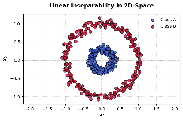

# Fit Perceptron
linear_model_2d = Perceptron(max_iter=1000, random_state=42)
linear_model_2d.fit(X, y)

w1, w2 = linear_model_2d.coef_[0]
b = linear_model_2d.intercept_[0]

print(f" Fitted line : {w1:.2f}$x_1$ + {w2:.2f}$x_2$ + {b:.2f} = 0")
print(" ")

line_x1 = np.linspace(-15, 15, 500)
line_x2 = -(w1 * line_x1 + b) / w2

plt.figure(figsize=(6, 4))
plt.plot(line_x1, line_x2, color='black', linestyle='-', linewidth=3,
         label=f"Fitted Line")

plt.scatter(X[y == 1, 0], X[y == 1, 1], color='royalblue', label='Class ', edgecolors='k', s=30)
plt.scatter(X[y == -1, 0], X[y == -1, 1], color='crimson', label='Class B', edgecolors='k', s=30)

# 6. Zoom the camera out to a macro window so we can see both elements
plt.xlim(-12, 12)
plt.ylim(-12, 12)

# Structural markers
plt.axhline(0, color='gray', linestyle=':', alpha=0.5)
plt.axvline(0, color='gray', linestyle=':', alpha=0.5)
plt.grid(True, linestyle=':', alpha=0.5)
# plt.title(f"Macro View: Runaway Hyperplane Due to Symmetric Collapse\nAccuracy: {linear_model_2d.score(X, y)*100:.1f}%",
#           fontsize=12, fontweight='semibold', pad=15)
plt.xlabel(" $x_1$")
plt.ylabel(" $x_2$")
plt.legend(loc='upper right')
plt.axis('equal')

plt.tight_layout()
plt.show()

# --- Output ---
# Fitted line : -0.26$x_1$ + -0.26$x_2$ + 1.00 = 0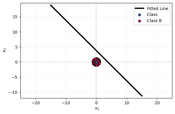

start_time = time.perf_counter()

x1 = X[:, 0]
x2 = X[:, 1]

# Apply the quadratic mapping function: \Phi(x) = [x1^2, \sqrt{2}*x1*x2, x2^2]
phi_1 = x1**2
phi_2 = np.sqrt(2) * x1 * x2
phi_3 = x2**2

# Stack into a new 3D feature array [N, 3]
X_explicit_3d = np.vstack((phi_1, phi_2, phi_3)).T

linear_model_3d = Perceptron(max_iter=100, random_state=42)
linear_model_3d.fit(X_explicit_3d, y)

# Stop timer
end_time = time.perf_counter()
explicit_compute_time = end_time - start_time

preds_3d = linear_model_3d.predict(X_explicit_3d)
acc_3d = accuracy_score(y, preds_3d)

print(f"Linear Perceptron Accuracy in explicitly mapped 3D space: {acc_3d * 100:.2f}%")
print(f"Explicit 3D Computation & Training Time: {explicit_compute_time:.6f} seconds\n")

fig = plt.figure(figsize=(10, 8))
ax = fig.add_subplot(1, 1, 1, projection='3d')

ax.scatter(X_explicit_3d[y==1, 0], X_explicit_3d[y==1, 1], X_explicit_3d[y==1, 2],
           color='royalblue', label='Class A', edgecolors='k', alpha=0.7, s=40)
ax.scatter(X_explicit_3d[y==-1, 0], X_explicit_3d[y==-1, 1], X_explicit_3d[y==-1, 2],
           color='crimson', label='Class B ', edgecolors='k', alpha=0.7, s=40)

# Extract weights and intercept
w1, w2, w3 = linear_model_3d.coef_[0]
b = linear_model_3d.intercept_[0]

# Generate a grid mesh over the first two feature coordinates (phi_1 and phi_2)
phi1_range = np.linspace(X_explicit_3d[:, 0].min() - 0.1, X_explicit_3d[:, 0].max() + 0.1, 20)
phi2_range = np.linspace(X_explicit_3d[:, 1].min() - 0.1, X_explicit_3d[:, 1].max() + 0.1, 20)
mesh_phi1, mesh_phi2 = np.meshgrid(phi1_range, phi2_range)

# Rearrange the hyperplane equation to calculate the height coordinate (phi_3):
# phi_3 = -(w1*phi_1 + w2*phi_2 + b) / w3
mesh_phi3 = -(w1 * mesh_phi1 + w2 * mesh_phi2 + b) / w3


plane_surface = ax.plot_surface(mesh_phi1, mesh_phi2, mesh_phi3,
                                 alpha=0.25, color='green', edgecolor='none')
plane_proxy = plt.Rectangle((0,0), 1, 1, fc="green", alpha=0.25)

ax.set_title(f"3D Linearly Separable Space\nAccuracy: {acc_3d*100:.1f}% | Time: {explicit_compute_time:.5f}s",
             fontsize=12, fontweight='semibold', pad=15)
ax.set_xlabel("$\phi_1 = x_1^2$")
ax.set_ylabel("$\phi_2 = \sqrt{2}x_1x_2$")
ax.set_zlabel("$\phi_3 = x_2^2$")

handles, labels = ax.get_legend_handles_labels()
handles.append(plane_proxy)
labels.append(f"Separating Plane: {w1:.2f}$\phi_1$ + {w2:.2f}$\phi_2$ + {w3:.2f}$\phi_3$ + {b:.2f} = 0")
ax.legend(handles=handles, labels=labels, loc='upper left')

# Adjust camera perspective angle for optimal visual separation
ax.view_init(elev=150, azim=30)

plt.tight_layout()
plt.show()

# --- Output ---
# Linear Perceptron Accuracy in explicitly mapped 3D space: 100.00%
# Explicit 3D Computation & Training Time: 0.003874 seconds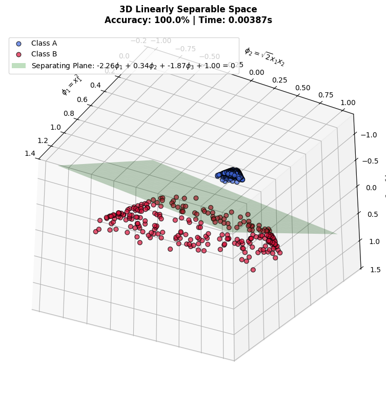

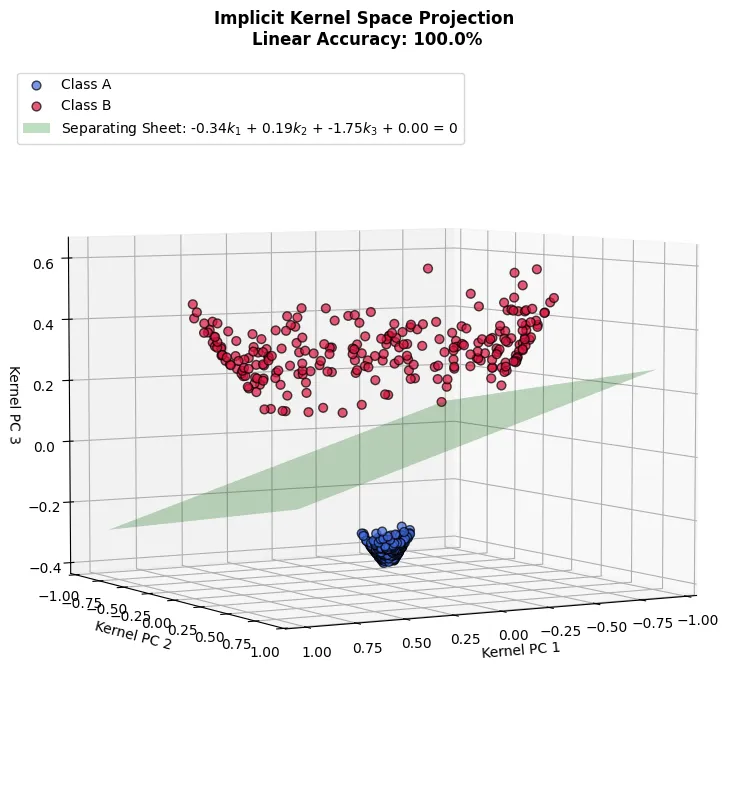
# Kernel Trick (Kernel-PCA)

def homogeneous_polynomial_kernel(X1, X2, degree=2):
    return (np.dot(X1, X2.T)) ** degree

K = homogeneous_polynomial_kernel(X, X, degree=2)


# Center the Gram Matrix
N = K.shape[0]
one_N = np.ones((N, N)) / N
K_centered = K - one_N.dot(K) - K.dot(one_N) + one_N.dot(K).dot(one_N)

# Compute Eigen-decomposition
eigenvalues, eigenvectors = np.linalg.eigh(K_centered)

# Sort eigenvalues and eigenvectors in descending order
idx = np.argsort(eigenvalues)[::-1]
eigenvalues = eigenvalues[idx]
eigenvectors = eigenvectors[:, idx]

# Project the data points onto the top 3 principal components of the kernel space [N x 3]
# We scale the coordinates by the square root of their respective eigenvalues
X_kernel_space_3d = eigenvectors[:, :3] * np.sqrt(np.abs(eigenvalues[:3]))

# Train our linear Perceptron on these implicit kernel-space coordinates
linear_model_kernel = Perceptron(max_iter=100, random_state=42)
linear_model_kernel.fit(X_kernel_space_3d, y)
acc_kernel = linear_model_kernel.score(X_kernel_space_3d, y)

print(f"Perceptron Accuracy in implicit Kernel Space: {acc_kernel * 100:.2f}%\n")



fig = plt.figure(figsize=(10, 8))
ax = fig.add_subplot(1, 1, 1, projection='3d')

# Scatter the kernel space coordinates
ax.scatter(X_kernel_space_3d[y==1, 0], X_kernel_space_3d[y==1, 1], X_kernel_space_3d[y==1, 2],
           color='royalblue', label='Class A ', edgecolors='k', alpha=0.7, s=40)
ax.scatter(X_kernel_space_3d[y==-1, 0], X_kernel_space_3d[y==-1, 1], X_kernel_space_3d[y==-1, 2],
           color='crimson', label='Class B ', edgecolors='k', alpha=0.7, s=40)

# Extract weights and intercept
w1, w2, w3 = linear_model_kernel.coef_[0]
b = linear_model_kernel.intercept_[0]

k1_range = np.linspace(X_kernel_space_3d[:, 0].min() - 0.05, X_kernel_space_3d[:, 0].max() + 0.05, 20)
k2_range = np.linspace(X_kernel_space_3d[:, 1].min() - 0.05, X_kernel_space_3d[:, 1].max() + 0.05, 20)
mesh_k1, mesh_k2 = np.meshgrid(k1_range, k2_range)

# Calculate the third kernel axis plane dimension (k3): k3 = -(w1*k1 + w2*k2 + b) / w3
mesh_k3 = -(w1 * mesh_k1 + w2 * mesh_k2 + b) / w3

# Plot the separating surface plane
plane_surface = ax.plot_surface(mesh_k1, mesh_k2, mesh_k3, alpha=0.25, color='green', edgecolor='none')
plane_proxy = plt.Rectangle((0,0), 1, 1, fc="green", alpha=0.25)

# Axis configurations using raw strings
ax.set_xlabel(r"Kernel PC 1")
ax.set_ylabel(r"Kernel PC 2")
ax.set_zlabel(r"Kernel PC 3")

# Combine legend structures
handles, labels = ax.get_legend_handles_labels()
handles.append(plane_proxy)
labels.append(f"Separating Sheet: {w1:.2f}$k_1$ + {w2:.2f}$k_2$ + {w3:.2f}$k_3$ + {b:.2f} = 0")
ax.legend(handles=handles, labels=labels, loc='upper left')

ax.set_title(f"Implicit Kernel Space Projection \nLinear Accuracy: {acc_kernel*100:.1f}%",
             fontsize=12, fontweight='semibold', pad=15)

# Adjust camera view position
ax.view_init(elev=5, azim=60)

plt.tight_layout()
plt.show()

# --- Output ---
# Perceptron Accuracy in implicit Kernel Space: 100.00%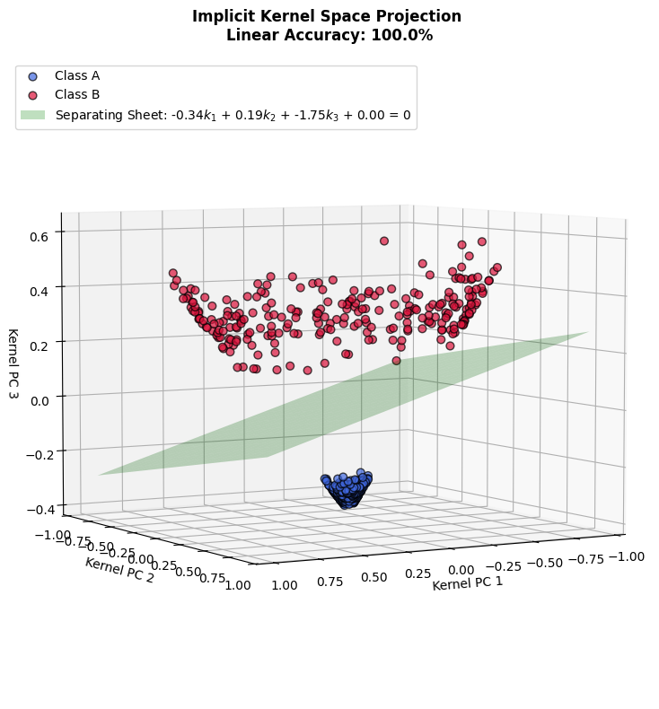

# The Infinite-Dimensional RBF Kernel
from sklearn.svm import SVC

start_rbf_time = time.perf_counter()


def rbf_kernel(X1, X2, gamma=5.0):
    """
    Computes the Radial Basis Function (Gaussian) Kernel Matrix.
    Formula: K(x, z) = exp(-gamma * ||x - z||^2)
    """
    # Vectorized computation of squared Euclidean distances between all rows
    sq_dists = np.sum(X1**2, axis=1, keepdims=True) + np.sum(X2**2, axis=1) - 2 * np.dot(X1, X2.T)
    return np.exp(-gamma * sq_dists)

# Compute the N x N training Gram Matrix using our custom RBF function
K_train = rbf_kernel(X, X, gamma=5.0)

# Train a Support Vector Classifier using our custom precomputed RBF kernel matrix
clf_rbf = SVC(kernel='precomputed')
clf_rbf.fit(K_train, y)

end_rbf_time = time.perf_counter()
rbf_compute_time = end_rbf_time - start_rbf_time

preds_rbf = clf_rbf.predict(K_train)
acc_rbf = accuracy_score(y, preds_rbf)

print(f"RBF Kernel Classifier Accuracy: {acc_rbf * 100:.2f}%")
print(f"RBF Execution & Training Time: {rbf_compute_time:.6f} seconds\n")

# --- Output ---
# RBF Kernel Classifier Accuracy: 100.00%
# RBF Execution & Training Time: 0.040846 seconds

Conclusion

Kernel methods introduced one of the most beautiful ideas in machine learning:

• Instead of explicitly transforming data into a higher-dimensional space, we can compute similarities as if the transformation had already occurred.
• The idea of "Kernel Trick" made nonlinear learning computationally feasible and laid the foundation for many modern machine learning algorithms.

References

1. Campbell, C. (2001). An introduction to kernel methods. Studies in Fuzziness and Soft Computing, 66, 155-192.
2. https://www.youtube.com/watch?v=IzGS8uKc5E4&list=PLD93kGj6_EdrkNj27AZMecbRlQ1SMkp_o&index=1
3. https://medium.com/@qjbqvwzmg/kernel-methods-in-machine-learning-theory-and-practice-b030bbe0eacc